Image Derivative
Taking the derivative of an image is a concept that I’ve seen come up both in edge detection and in computing optical flow. It’s confused the heck out of me because I would normally think of derivatives in terms of taking the derivative of a continuous function. However, with an image, you have a 2D matrix of seemingly random values, so what could it mean to take the derivative?
When taking the derivative of an image, you’re actually taking what’s called a discrete derivative, and it’s more of an approximation of the derivative. One simple example is that you can take the derivative in the x-direction at pixel x1 by taking the difference between the pixel values to the left and right of your pixel (x0 and x2).
I think it’s easiest to see how the image derivative is useful in locating edges. The derivative of a function tells you the rate of change, and an edge constitutes a high rate of change.
Sources
There are a number of sources I’ve used for learning about this topic.
University of Central Florida (UCF) Lecture on YouTube
-
The discussion of image derivatives starts at about 6:00 and runs till 17:45 in the video.
University of Nevada, Reno (UNR) Lecture Slides
-
The discussion of derivatives goes from slide 35 to the end.
Wikipedia
-
Prewitt Operator: http://en.wikipedia.org/wiki/Prewitt_operator
- This is the operator Dr. Shah discusses in the YouTube lecture.
Notes
Dr. Shah’s video lecture begins with a quick refresher on the definition of a derivative in Calculus. In calculus we have continuous valued functions, but with images we have discrete data.
The first equation below shows the calculus definition of a derivative. With image data, the smallest possible delta x is 1, so we use the second and third equations to approximate the derivative.
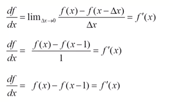
Taking the difference between x and x-1 is just one possibility, and is called the “backward difference”. The other options are:

An image actually has three variables, an x-coordinate, a y-coordinate, and an intensity. So the derivative of an image has two dimensions. We can take the derivative in the x direction and in the y direction, and together these make up the “gradient vector”:

[at 13:31 in the video]
Going back to edge detection, the gradiant direction gives you the normal to the edge (it’s perpindicular to the edge), and the gradient magnitude gives you the strength of the edge.
To compute the derivative with respect to x at a given pixel, it sounds like in practice, to reduce the affects of noise, we:
-
Use the “central difference”
-
Average the derivative of the pixel with that of the row above and row below:
**
[15:07]
Apply the mask by multiplying each component of the matrix with the corresponding pixel value (the pixel of interest is at the center of the matrix) and sum them all up.
Again, we could just use the middle row for fx and the middle column for fy, but we include the surrounding pixels to help reduce the affect of noise.
We can’t apply the mask to the border pixels so we don’t, the derivative at those pixels is set to 0.

He doesn’t mention this until he talks about edge detectors later on, but the derivative mask he’s using here is called the Prewitt operator, and you can read more about it on Wikipedia: http://en.wikipedia.org/wiki/Prewitt_operator. The Prewitt operator omitts the 1/3, I’m guessing for the sake of computational efficiency.
Both lectures provide the following image as an example of the derivative with respect to x and y.

Notice how, in the df/dx image, the vertical boundary between her face and hair is more apparent, or similarly the vertical boundary between her hair and the wall. The df/dy image, on the other hand, accentuates horizontal edges like the side/top of her hand, the edge of her eyes, and her eyebrows.
The significance of the greyscale values in these images had me confused for a while. The reason the images are mostly grey is that the value of the derivative actually ranges from -255 to 255, but to visualize it we must scale this to the range 0 to 255. So anywhere the derivative is zero (no edge), it’s given the value 128 (a neutral grey).
Also notice how, in the df/dx image, a horizontal transition from light to dark (like the side of her face) is colored white, while a dark to light transition (like on her hand) is colored black.
We measure the strength of an edge by combining the df/dx and df/dy values, as shown below.

Again, the grayscale values in the final image caused me some confusion. If most of the pixel values are about 128, how does the final image end up mostly black? The pixel values in the final image (the gradient magnitude values) are computed using the original derivative values ranging from -255 to 255. So in the final image, areas with no edges are black, and areas with edges (light to dark transitions or dark to light transitions) are colored white.