UCF Lecture 6 - Optical Flow

30 Mar 2013

The following post contains my notes on lecture 6 of Dr. Shah’s computer vision course:

http://www.youtube.com/watch?v=5VyLAH8BhF8

Optical flow is the motion of a single pixel from one frame to the next.

Optical flow is used for:

Motion based segmentation:
- Identifying objects in the scene based on their movement versus the stationary background (the object is moving, but the background is not).
“Structure from motion”
- Retrieving 3D data about an object from its movement.
- Recall the video in the first lecture of balls representing a person’s joints–our brain can recognize this as a person based on the motion.
Alignment
- Video stabilization (removing camera shake)
- Video from moving camera (like a UAV, again recall video from lecture 1)
Video compression
- Apply displacement to one image to synthesize the next, encode any difference/uniqueness.

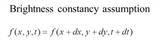
Brightness Constantancy Assumption

Horn & Schunk

Horn is a famous MIT vision researcher, Brian Schunk was his PhD student.

They came up with the basic optical flow concept.

Brightness constancy assumption: If you take the frames very close together (30fps), a pixel will move slightly but it’s brightness will not change by much (because it’s only been 1/30s).

****

[10:30]

###

Taylor Series Approximation

We’re going to take the taylor series approximation of the above equation.

I found the equations on Wikipedia to be slightly clearer than the ones Dr. Shah uses.

I(x + dx, y + dy, t + dt) = The brightness (intensity) of a pixel at its new location in frame 2.
I(x, y, t) = The brightness (intensity) of a pixel in its location in frame 1.

This equation only shows the first two terms of the taylor series (only the first derivative). The other terms must not be significant.

This equation just states that the intensity of a pixel in frame 2 is equal to it’s intensity in frame 1 + a small change.

The first term, dI / dx * delta x

dI / dx = The rate of change in intensity relative to the x axis.

Multiplied by the small change in x gives you a small difference in intensity.

We are making the assumption that the pixel brightness is constant, so we’re assuming:

Subtituting this into our Taylor series approximation above, we find that:

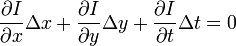
The above equation simply states that the change in pixel intensity is 0 (between the first and second frames, and with the small amount of motion of the pixel).

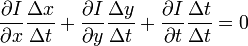
We said that the pixel is moving a small amount, dx and dy, between the two frames. And the two frames are separated in time by dt. So we can find the pixel’s velocity in the x direction as dx/dt, and the its velocity in the y direction as dy/dt.

To do this, we divide the equation by dt and we get:

We write the x component of the velocity as Vx and the y component as Vy. We also remove dt / dt, leaving us with:

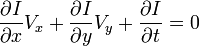
Finally, another notation for “the derivative of I with respect to x” is Ix, so we have:

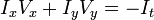
In the video lecture, he uses ‘u’ for Vx and ‘v’ for Vy

It’s important to know that given two sequential image frames it is possible to compute Ix, Iy, and It. However, Vx and Vy are unknown. Which is simply to say that for a given pixel in the first frame we don’t know where it will end up in the next frame.

Normal Flow & Parallel Flow

[15:00]

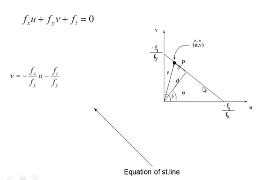
We have two unknowns, u and v. But we can write this as a linear equation, and we at least know that the u and v will lie somewhere on the line as shown above.

We do know that the vector (u, v) is equal to the vectors p + d

d is called “normal flow”
p is called “parallel flow”

We can derive that d in the above figure is equal to:

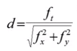
[16:31]

So we know ‘d’, but we dont’ know ‘p’.

Note: He never comes back to this notion of ‘p’ and ‘d’, so I’m not sure why they’re included in the discussion. It seems sufficient to understand that Vx and Vy are unknowns, and that we need to add an additional constraint to the problem in order to solve for them.

Adding a Smoothness Constraint

[17:40]

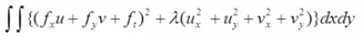
Horn & Schunk treated this (not knowing ‘p’) as an optimization problem.

The double integral means we’re doing this for every pixel.
The first term:
- This is the brightness constancy function, which we’ve said is ideally 0.
- It may not be exactly 0, though, there may be a small error, so we square the error and get a small number for this term.
The second term:
- This is adding a smoothness constraint, the idea being that if the object is moving, all of the pixels in the object will have similar motion.
- Object boundaries will be a problem, though (this only kind of makes sense to me).
- Take the derivative of the velocity. If the change is smooth, then these derivatives will again be small values. (Again, I’m not very clear on this)
Ideally both terms should be small. So the idea is to minimize this function (find its minimum). He decides to not go into a lot of detail on the math
- At a peak or valley in a function, the derivative is equal to 0. So to minimize a function, you take its derivative and equate it 0, then solve the equation.
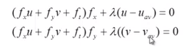
- If you take the above equation and take the derivative with respect to u and equate that to 0, and also take the derivative with respect to v and set that to 0, you get the following two functions:

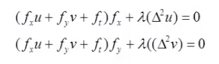
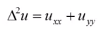
The second term we recognize as the Laplacian, which is equal to the second derivative of u with respect to x plus the second derivative of u with respect to y.

[22:27]

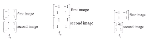
Derivative Masks

He shows the Derivative masks used by a researcher named Roberts. They’re similar to the masks we saw in the lecture on edge detection. The ft mask is a new concept, though.

****

[24:37]

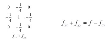
Laplacian Mask

This is a new concept.

****

[25:38]

Take the average of the four neighbors (multiply each neighbor by 1/4) and subtract that average from the value of the central pixel.

Using this approximation for the Laplacian, we can re-write the earlier smoothness equation:

[26:20]

Now we have two equations for u and v, and we have all of the other values, so we can solve for u and v as:

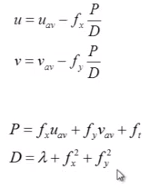
[27:15]

There is a step now that I don’t understand. You start with initial values of u = 0 and v = 0, then “iterate”. Does iteration refer to going over subsequent frames? I don’t think so, the implication seems to be multiple iterations of a single frame.

Lucas & Kanade (Least Squares)

[31:00]

Optical flow dates back to 1980s, many more advancements have been made since.

Kanade - famous researcher, Lucas was his student.

[33:20]

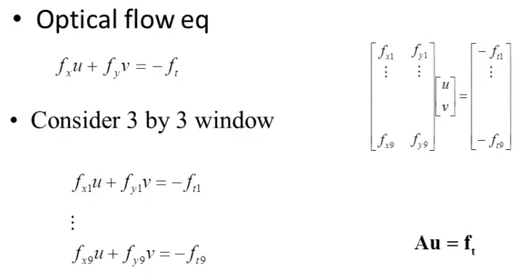
Take a 3x3 window, and assume that all of the pixels have the same x and y velocity.

Now we have 9 equations and two unknowns.

The equations can be represented as a matrix as shown.

We representl the matrix on the left as ‘A’.

[35:13]

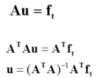
We need to solve for ‘u’, but it’s not possible to divide both sides by A.

It’s not possible (?) to take the inverse of a matrix that isn’t square.

But If you multiply the 9x2 matrix by its 2x9 transpose, you get a 2x2 matrix. That allows to separate out the ‘u’ term, giving us the equation above.

The three ‘A’ terms in the final equation are referred to as the ‘pseudo-inverse’, apparently this is a common concept.

Least Squares Fit

[37:20]

Once we have u and v, ideally the optical flow equation at each pixel in the window should equal 0. In practice, there will be some small error at each pixel.

The optimum value for u and v will minimize this error. This is expressed by the following equation.

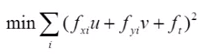
Note that squaring the error means that larger errors will contribute an exponentially larger amount to the total than smaller errors.

To minimize these functions we take the derivative, once with respect to u and again with respect to v, and set both equations to 0.

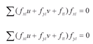
[36:27]

The summations can be expanded to:

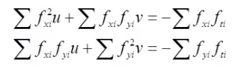
Then rewritten in matrix form as:

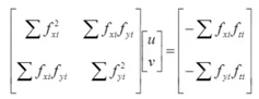
This 2x2 matrix can be inverted, giving us:

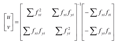
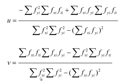
Expanding this with the definition of a matrix inverse, and writing the equations for u and v separately, we have:

****

[41:03]

Lucas-Kanade With Pyramids

The Lucas-Kanade method fails when the motion is large, for example if a pixel moves 15 pixels from one frame to the next. The reason Dr. Shah gives is that the derivative mask is only 2x2 pixels.

The solution to this is something called pyramids.

Make multiple scales of the image.

* The 16 pixel motion will become a 1 pixel motion if you scale the image down by 16.