AdaBoost Tutorial
My education in the fundamentals of machine learning has mainly come from Andrew Ng’s excellent Coursera course on the topic. One thing that wasn’t covered in that course, though, was the topic of “boosting” which I’ve come across in a number of different contexts now. Fortunately, it’s a relatively straightforward topic if you’re already familiar with machine learning classification.
Whenever I’ve read about something that uses boosting, it’s always been with the “AdaBoost” algorithm, so that’s what this post covers.
AdaBoost is a popular boosting technique which helps you combine multiple “weak classifiers” into a single “strong classifier”. A weak classifier is simply a classifier that performs poorly, but performs better than random guessing. A simple example might be classifying a person as male or female based on their height. You could say anyone over 5’ 9” is a male and anyone under that is a female. You’ll misclassify a lot of people that way, but your accuracy will still be greater than 50%.
AdaBoost can be applied to any classification algorithm, so it’s really a technique that builds on top of other classifiers as opposed to being a classifier itself.
You could just train a bunch of weak classifiers on your own and combine the results, so what does AdaBoost do for you? There’s really two things it figures out for you:
- It helps you choose the training set for each new classifier that you train based on the results of the previous classifier.
- It determines how much weight should be given to each classifier’s proposed answer when combining the results.
Training Set Selection
Each weak classifier should be trained on a random subset of the total training set. The subsets can overlap–it’s not the same as, for example, dividing the training set into ten portions. AdaBoost assigns a “weight” to each training example, which determines the probability that each example should appear in the training set. Examples with higher weights are more likely to be included in the training set, and vice versa. After training a classifier, AdaBoost increases the weight on the misclassified examples so that these examples will make up a larger part of the next classifiers training set, and hopefully the next classifier trained will perform better on them.
The equation for this weight update step is detailed later on.
Classifier Output Weights
After each classifier is trained, the classifier’s weight is calculated based on its accuracy. More accurate classifiers are given more weight. A classifier with 50% accuracy is given a weight of zero, and a classifier with less than 50% accuracy (kind of a funny concept) is given negative weight.
Formal Definition
To learn about AdaBoost, I read through a tutorial written by one of the original authors of the algorithm, Robert Schapire. The tutorial is available here.
Below, I’ve tried to offer some intuition into the relevant equations.
Let’s look first at the equation for the final classifier.

The final classifier consists of ‘T’ weak classifiers. h_t(x) is the output of weak classifier ‘t’ (in this paper, the outputs are limited to -1 or +1). Alpha_t is the weight applied to classifier ‘t’ as determined by AdaBoost. So the final output is just a linear combination of all of the weak classifiers, and then we make our final decision simply by looking at the sign of this sum.
The classifiers are trained one at a time. After each classifier is trained, we update the probabilities of each of the training examples appearing in the training set for the next classifier.
The first classifier (t = 1) is trained with equal probability given to all training examples. After it’s trained, we compute the output weight (alpha) for that classifier.

The output weight, alpha_t, is fairly straightforward. It’s based on the classifier’s error rate, ‘e_t’. e_t is just the number of misclassifications over the training set divided by the training set size.
Here’s a plot of what alpha_t will look like for classifiers with different error rates.

There are three bits of intuition to take from this graph:
-
The classifier weight grows exponentially as the error approaches 0. Better classifiers are given exponentially more weight.
-
The classifier weight is zero if the error rate is 0.5. A classifier with 50% accuracy is no better than random guessing, so we ignore it.
-
The classifier weight grows exponentially negative as the error approaches 1. We give a negative weight to classifiers with worse worse than 50% accuracy. “Whatever that classifier says, do the opposite!”.
After computing the alpha for the first classifier, we update the training example weights using the following formula.

The variable D_t is a vector of weights, with one weight for each training example in the training set. ‘i’ is the training example number. This equation shows you how to update the weight for the ith training example.
The paper describes D_t as a distribution. This just means that each weight D(i) represents the probability that training example i will be selected as part of the training set.
To make it a distribution, all of these probabilities should add up to 1. To ensure this, we normalize the weights by dividing each of them by the sum of all the weights, Z_t. So, for example, if all of the calculated weights added up to 12.2, then we would divide each of the weights by 12.2 so that they sum up to 1.0 instead.
This vector is updated for each new weak classifier that’s trained. D_t refers to the weight vector used when training classifier ‘t’.
This equation needs to be evaluated for each of the training samples ‘i’ (x_i, y_i). Each weight from the previous training round is going to be scaled up or down by this exponential term.
To understand how this exponential term behaves, let’s look first at how exp(x) behaves.
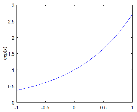
The function exp(x) will return a fraction for negative values of x, and a value greater than one for positive values of x. So the weight for training sample i will be either increased or decreased depending on the final sign of the term “-alpha * y * h(x)”. For binary classifiers whose output is constrained to either -1 or +1, the terms y and h(x) only contribute to the sign and not the magnitude.
y_i is the correct output for training example ‘i’, and h_t(x_i) is the predicted output by classifier t on this training example. If the predicted and actual output agree, y * h(x) will always be +1 (either 1 * 1 or -1 * -1). If they disagree, y * h(x) will be negative.
Ultimately, misclassifications by a classifier with a positive alpha will cause this training example to be given a larger weight. And vice versa.
Note that by including alpha in this term, we are also incorporating the classifier’s effectiveness into consideration when updating the weights. If a weak classifier misclassifies an input, we don’t take that as seriously as a strong classifier’s mistake.
Practical Application
One of the biggest applications of AdaBoost that I’ve encountered is the Viola-Jones face detector, which seems to be the standard algorithm for detecting faces in an image. The Viola-Jones face detector uses a “rejection cascade” consisting of many layers of classifiers. If at any layer the detection window is _not _recognized as a face, it’s rejected and we move on to the next window. The first classifier in the cascade is designed to discard as many negative windows as possible with minimal computational cost.
In this context, AdaBoost actually has two roles. Each layer of the cascade is a strong classifier built out of a combination of weaker classifiers, as discussed here. However, the principles of AdaBoost are also used to find the best features to use in each layer of the cascade.
The rejection cascade concept seems to be an important one; in addition to the Viola-Jones face detector, I’ve seen it used in a couple of highly-cited person detector algorithms (here and here). If you’re interested in learning more about the rejection cascade technique, I recommend reading the original paper, which I think is very clear and well written. (Note that the topics of Haar wavelet features and integral images are not essential to the concept of rejection cascades).