Stereo Vision Tutorial - Part I
This tutorial provides an introduction to calculating a disparity map from two rectified stereo images, and includes example MATLAB code and images.
A note on this tutorial: This tutorial is based on one provided by Mathworks a while back. It’s no longer on their website, but I’ve found an archived version here. If that goes down for some reason, I’ve also saved it as a PDF here. You can find my code and the example images at the bottom of this post; the code I provide does not have any dependencies on the computer vision toolbox.
Simple Block Matching
With stereo cameras, objects in the cameras’ field of view will appear at slightly different locations within the two images due to the cameras’ different perspectives on the scene.
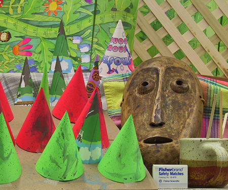
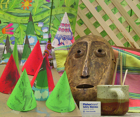
Below are two stereo images from the “Cones” dataset created by Daniel Scharstein, Alexander Vandenberg-Rodes, and Rick Szeliski. Their dataset is available here.
Left Image:

Right Image:

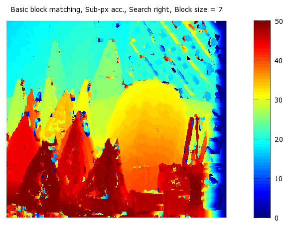
Depth information can be computed from a pair of stereo images by first computing the distance in pixels between the location of a feature in one image and its location in the other image. This gives us a “disparity map” such as the one below. It looks a lot like a depth map because pixels with larger disparities are closer to the camera, and pixels with smaller disparities are farther from the camera. To actually calculate the distance in meters from the camera to one of those cones, for example, would require some additional calculations that I won’t be covering in this post.

According to the Matlab tutorial, a standard method for calculating the disparity map is to use simple block matching. Essentially, we’ll be taking a small region of pixels in the right image, and searching for the closest matching region of pixels in the left image.
For example, we’ll take the region of pixels within the black box in the left image:

And find the closest matching block in the right image:
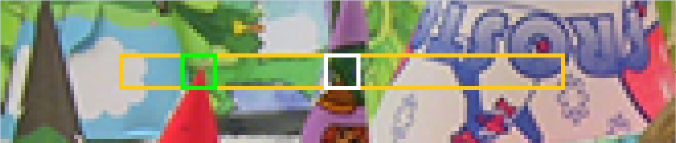
When searching the right image, we’ll start at the same coordinates as our template (indicated by the white box) and search to the left and right up to some maximum distance. The closest matching block is the green box in the second image. The disparity is just the horizontal distance between the centers of the green and white boxes.
Block Comparison
What is our similarity metric for finding the “closest matching block”? It’s simpler than you might think, it’s a simple operation called “sum of absolute differences” or “SAD”.
Before computing the disparity map, we convert the two images to grayscale so that we only have one value (0 - 255) for each pixel.
To compute the sum of absolute differences between the template and a block, we subtract each pixel in the template from the corresponding pixel in the block and take the absolute value of the differences. Then we sum up all of these differences and this gives a single value that roughly measures the similarity between the two image patches. A lower value means the patches are more similar.

To find the “most similar” block to the template, we compute the SAD values between the template and each block in the search region, then choose the block with the lowest SAD value.
Image Rectification
Note that we’re only searching horizontally for matching blocks and not vertically. As in the Matlab tutorial, we’ll be working with images which have already been “rectified”. Image rectification is important because it ensures that we only have to search horizontally for matching blocks, and not vertically. That is, a feature in the left image will be in the same pixel row in the right image.
I haven’t explored image rectification very deeply yet. Matlab has a tutorial, again in the computer vision toolbox, on how to perform image rectification. It involves finding a set of matching keypoints (using an algorithm such as SIFT or SURF) between the two images, and then applying transformations to the images to bring the keypoints into alignment. It’s not clear to me, however, whether this process is necessary if the images are taken with two well-aligned / well-calibrated cameras.
In any case, the “Cones” images we’re using are rectified.
Search Range and Direction
The block-matching algorithm requires us to specify how far away from the template location we want to search. I suppose this is based on the maximum disparity you expect to find in your images. The disparity in the “Cones” images appears to be much larger than in the images used by the Matlab tutorial–I manually inspected some points in the image and found that there are features which shift as many as 50 pixels.
The Matlab example code searches both to the left and right of the template for matching blocks, though intuitively you would think you only need to search in one direction. Mathworks explains this decision in the tutorial: “In general, slight angular misalignment of the stereo cameras used for image acquisition can allow both positive and negative disparities to appear validly in the depth map. In this case, however, the stereo cameras were near perfectly parallel, so the true disparities have only one sign.”
In the “Cones” images, the true disparities are only positive (shifted to the right). By only searching to the right, the code runs quicker (since it searches roughly half as many blocks) and actually produces a more accurate disparity map. Below, the first disparity map was generated by searching in both directions, and the second was generated by only searching to the right. Note that there is less noise in the cones in the second image.


Template Size
The Matlab tutorial uses a template size of 7x7 pixels. I experimented with different template sizes for the cone images. Larger templates generally appear to generate a less noisy disparity map, though at a higher compute cost. Also, note that some detail is lost in the lattice material in the background of the image.


Template Shape At Edges
The block matching code is pretty straightforward; the one bit of complexity comes from how we handle the pixels at the edges of the image. The way this is handled in the Matlab tutorial is that we crop the template to the maximum size that will fit without going past the edge of the image. For example, the default block / template size is 7x7 pixels. But for the pixel in the top left corner (row 1, column 1), we can’t include any of the pixels to the left or above, so we use a template that is only 4x4 pixels. For the pixel at row 2, column 1, we use a template that is 5 pixels tall and 4 pixels wide. The same shape and size is obviously used for the blocks as well.
Sub-pixel Estimation
The disparity values that we calculate using the block matching will all be integers, since they correspond to pixel offsets. It’s possible, though, to interpolate between the closest matching block and its neighbors to fine -tune the disparity value to a “sub-pixel” location. From the Matlab tutorial: “Previously we only took the location of the minimum cost as the disparity, but now we take into consideration the minimum cost and the two neighboring cost values. We fit a parabola to these three values, and analytically solve for the minimum to get the sub-pixel correction.”
I haven’t completely unpacked the math behind this, but here’s a simple example that should help illustrate the concept.
Below are three points, marked by red x’s, that are equally spaced in the x direction and all lie on a parabola.

Think of the middle x as like our closest matching block. It has the lowest y value of the three points, but it’s not actually at the minimum of the parabola. We can calculate (probably estimate?) the location of the parabola’s minimum using the following equation from the Matlab code. d2 is the disparity (pixel offset) of the closest matching block and d_est is our sub-pixel estimate of the actual disparity. C2 is the SAD value (or Cost) at the closest matching block, and C1 and C3 are the SAD values of the blocks to the left and right, respectively.
![]()
If you apply this equation to the three points on the above parabola, you get x_est ~= 0, which is plotted with the black circle.
Smoothing And Image Pyramids
There are two additional topics covered by the original MATLAB tutorial that I didn’t get to cover in detail in this post.
The first is a technique for improving the accuracy of the disparity map by taking into account the disparities of neighboring pixels. This is implemented using dynamic programming.
The final topic is image pyramiding which is a technique that can speed up the block matching process. It involves sub-sampling the image to quickly search at a coarse scale, then refining the search at a smaller scale.
Code
Simply save the following three files to a single directory, and cd to that directory before running ‘stereoDisparity’.
Note that the block matching process is extremely slow. It takes roughly 5 minutes to complete on my 3.4GHz Intel i7. This is partly due to the high disparity values present in the “Cones” images vs. the Matlab example. Also, the image pyramid technique discussed later on in the Mathworks tutorial should reduce the compute cost significantly.
Update, October 2016 - Where’s Part II?
For those looking for Part II of this tutorial, I’m sorry, it may never come. But! Before you lose hope! You can go look at the original material that I was using to understand this stuff. I found an archived copy of the original Mathworks article here. If that goes down for some reason, I’ve also saved it as a PDF here.
Finally, I do have my own commented version of the Dynamic Programming code which I can share with you here.