Deep Learning Tutorial - PCA and Whitening

Principal Component Analysis

PCA is a method for reducing the number of dimensions in the vectors in a dataset. Essentially, you’re compressing the data by exploiting correlations between some of the dimensions.

Covariance Matrix

PCA starts with computing the covariance matrix. I found this tutorial helpful for getting a basic understanding of covariance matrices (I only read a little bit of it to get the basic idea).

The following equation is presented for computing the covariance matrix.

Note that the placement of the transpose operator creates a matrix here, not a single value.

Note that this function only computes the covariance matrix if the mean is zero. The proper function would be based on (x - mu)(x - mu)^T. For the tutorial example, the dataset has been adjusted to have a mean of 0.

For 2D data, here are the equations for each individual cell of the 2x2 covariance matrix, so that you can get more of a feel for what each element represents.

If you subtract the means from the dataset ahead of time, then you can drop the “minus mu” terms from these equations. Subtracting the means causes the dataset to be centered around (0, 0).

The top-left corner is just a measure of how much the data varies along the x_1 dimension. Similarly, the bottom-right corner is the variance in the x_2 dimension.

The bottom-left and top-right corners are identical. These indicate the correlation between x_1 and x_2.

If the data is mainly in quadrants one and three, then all of the x_1 * x_2 products are going to be positive, so there’s a positive correlation between x_1 and x_2.

If the data is all in quadrants two and four, then the all of the products will be negative, so there’s a negative correlation between x_1 and x_2.

If the data is evenly dispersed in all four quadrants, then the positive and negative products will cancel out, and the covariance will be roughly zero. This indicates that there is _no _correlation.

Eigenvectors

After calculating the covariance matrix for the dataset, the next step is to compute the  eigenvectors of the covariance matrix. I found this tutorial helpful. Again, I only skimmed it and got a high level understanding.

The eigenvectors of the covariance matrix have the property that they point along the major directions of variation in the data.

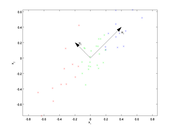
Why this is the case is beyond me. I suspect you’d have to be more intimately acquainted with how the eigenvectors are found in order to understand why they have this property. So I’m just taking it as a given for now.

Projecting onto an eigenvector

The tutorial explains that taking the dot product between a data point, x, and an eigen vector, u_1, gives you “the length (magnitude) of the projection of onto the vector . “

Take a look at the Wikipedia article on Scalar Projection to help understand what this means.

The resulting scalar value is a point along the line formed by the eigen vector.

What’s actually involved, then, in reducing a 256 dimensional vector down to 50 dimensional vector? You will be taking the dot product between your 256-dimensional vector x and each of the top 50 eigen vectors.

It was interesting to me to note that this is equivalent to evaluating a neural network with 256 inputs and 50 hidden units, but with no activation function on the hidden units (i.e., no sigmoid function).

Whitening

There are two things we are trying to accomplish with whitening:

1. Make the features less correlated with one another.

2. Give all of the features the same variance.

Whitening has two simple steps:

1. Project the dataset onto the eigenvectors. This rotates the dataset so that there is no correlation between the components.

2. Normalize the the dataset to have a variance of 1 for all components. This is done by simply dividing each component by the square root of its eigenvalue.

I asked a Neural Network expect I’m connected with, Pavel Skribtsov, for more of an explanation on why this technique is beneficial:

"This is a common trick to simplify optimization process to find weights. If the input signal has correlating inputs (some linear dependency) then the [cost] function will tend to have "river-like" minima regions rather than minima points in weights space. As to input whitening - similar thing - if you don't do it - error function will tend to have non-symmetrical minima "caves" and since some training algorithms have equal speed of update for all weights - the minimization may tend to skip good places in narrow dimensions of the minima while trying to please the wider ones. So it does not directly relate to deep learning. If your optimization process converges well - you can skip this pre-processing."

PCA in 2D Exercise

This exercise is pretty straightforward. A few notes, though:

• Note that you don’t need to adjust the data to have a mean of 0, it’s already close enough.

• In step 1a, where it plots the eigen vectors, your plot area needs to be square in order for it to look right. Mine was a rectangle at first (from a previous plot) and it threw me off–it made the second eigen vector look wrong.

  • The command axis(“square”) is supposed to do this, but for seem reason it gives my plot a 5:4 ratio, not 1:1. What a pain!

PCA and Whitening Exercise

• If you are using Octave instead of Matlab, there’s a modification you’ll need to make to line 93 of display_network.m. Remove the arguments ‘EraseMode’ and ‘none’.

• When subtracting the mean, the instructions say to calculate the mean per image, but the code says to calculate it per row (per pixel). This section of the tutorial describes why they compute it per image for natural images.

• You can use the command “colorbar” to add a color legend to the plot for the imagesc command.

Using 116 out of 144 principal components preserved 99% of the variance.

Here is the final output of my code, showing the original image patches and the whitened images.

Before whitening:

After whitening: