Deep Learning Tutorial - Self-Taught Learning & Deep Networks

This post covers the sections of the tutorial titled “Self-Taught Learning and Unsupervised Feature Learning” and “Building Deep Networks for Classification”.

Self-Taught Learning

In the self-taught learning section, we train an auto-encoder on the digits 5 - 9, then use this auto-encoder as a feature extractor for recognizing the digits 0 - 4. The exercise takes the training data for the digits 0 - 4 and divides them in half, with one half used for training and the other used for testing.

This is a straight-forward exercise that just involves combining some of the code that you’ve already written.

Note for Octave Users

I did run into some memory issues on this exercise using Octave.  There are a total of 29,404 examples of the digits 5 - 9 used to train the autoencoder, and my training code runs out of memory on this large of a dataset. To work around this, I randomly selected 10,000 examples using ‘randperm’, and trained the autoencoder on just these 10k examples. I still got 98.28% accuracy overall, so this didn’t appear to affect the accuracy too dramatically.

Deep Networks

In the deep networks exercise, you’ll be building a deep MLP which achieves impressive performance on the handwritten digits dataset.

The deep network will consist of two stacked autoencoders with 200 neurons each, followed by a Softmax Regression classifier on the output.

The key step in this exercise will be the fine-tuning of the network to improve its overall accuracy. During the fine tuning step, you’ll be treating the network as a regular MLP network without the sparsity constraints on the hidden layers. In other words, you’ll be using ordinary backpropogation to train the network on the labeled dataset.

Note that the output layer (the Softmax classifier) has already been optimized over the training set. The real intent of the ‘fine-tuning’ step is to tweak the parameters in the autoencoder layers to improve performance. Of course, the softmax parameters will be updated as well as we adjust the earlier layers.

My implementation achieved 92.05% accuracy on the test set prior to fine-tuning, and 98.13% accuracy after fine-tuning. This is a pretty dramatic improvement! Looking at the performance table on the MNIST website, 92.05% is pretty poor. This seems to suggest that the auto-encoders alone aren’t fantastic feature extractors, and that the autoencoder technique just provides very good initial weight values to use in training the deep MLP. Really, it’s the ordinary backprop training that produces the strong performance, the autoencoder training steps just give the backprop training a good head-start.

Backpropagation

The tutorial notes on backpropagation provide a nice summary of the equations you need to implement. However, there is a key difference, which is that we are using the logarithmic cost function instead of the mean-squared error.

Log cost

When calculating the cost, use the same cost function which you used in the Softmax regression exercise.

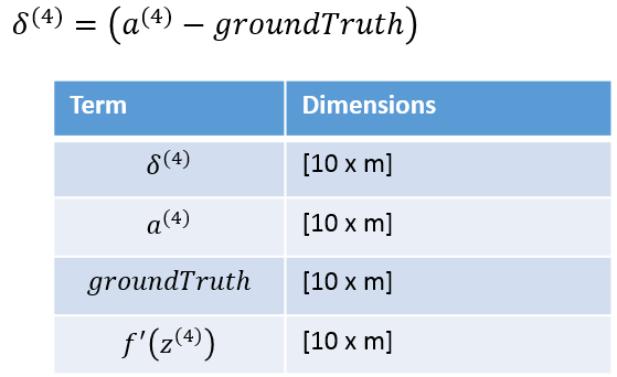
This also affects the delta term for the output layer. Using the MSE cost, this term is given by:

But when using the log cost, we’ll drop that sigmoid prime term. See my equations below.

Bias terms

One of the trickier bits of implementing back propagation is keeping track of the bias term. Remember that in the notation the weight matrix ‘W’ does not include the bias term. The bias term is stored sepearately as the vector ‘b’.  ’Theta’, however, includes both W and b.

Also, the starter code for the Softmax Regression exercise doesn’t seem to be set up to include a bias term. I implemented Softmax Regression without a bias term and it seems to work fine. It could be that the Softmax classifier is able to learn its model without a bias term, or it could be that it’s just able to learn reasonable parameters even without the bias. In any case, if you have a bias term in your softmax parameters, you may need to modify my equations slightly.

Equations for gradients

In the equations below, ‘m’ is the number of training examples.

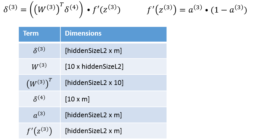
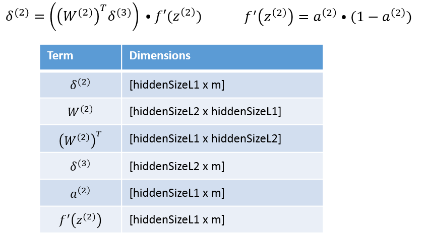
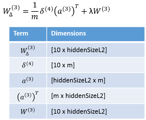
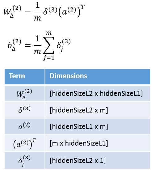
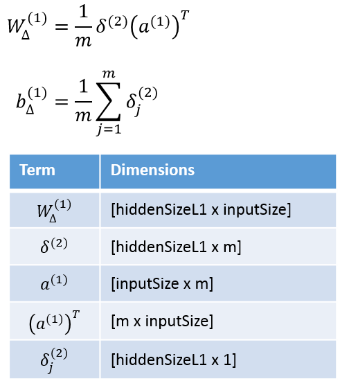
I’ve found that, to vectorize Matlab code, the best approach is to look at the dimensions of the matrices to ensure that the dimensions all line up. If the dimensions match up correctly, you’ve probably implemented the equation correctly. Under each equation you’ll find a table showing the matrix dimensions [rows x columns] for each term in the equation.

Delta Terms

The first step is to calculate the delta terms, working backwards from the output layer.

I got the equation for the output layer delta term from the backprop assignment in the Coursera course on Machine Learning, where we also used the log cost.

You could probably also derive this equation by working through the derivative of the cost function to verify this.

The gradient checking code verified my implementation.

In calculating the layer 3 and layer 2 deltas, note that W does not include the bias term, and neither does a.

Gradients

Once you have the delta terms, you can calculate the gradient values.

My Softmax Regression model doesn’t include a bias term, so I’m only showing the equation for gradients for W. Also, note that we are applying regularization to the output layer, and so I’ve included the lambda term.

For the hidden layers, I do have a bias term. Also, we are not applying regularization to these layers, so there is no lambda term.

Note for Octave Users

I am looking at purchasing Matlab, and currently have a trial version which I used to complete this exercise.

I think that you should still be able to complete this exercise using Octave, but you may just need to use a smaller training set size for the auto-encoders. For example, you could try training on a random selection of 10,000 images instead of the full 60,000. The final accuracy of your system may not be as good, but you should still be able to implement it and verify it’s correctness using the gradient checking code they provide.