RBFN Tutorial Part II - Function Approximation

A number of people have asked me, in response to my tutorial on Radial Basis Function Networks (RBFNs) for classification, about how you would apply an RBFN to function approximation or regression (and for Matlab code to do this, which you can find at the end of the post).

In fact, classification is really just a specific case of function approximation. In classification, the function you are trying to approximate is a score (from 0 to 1) for a category.

Below is a simple example of an RBFN applied to a function approximation problem with a 1 dimensional input. A dataset of 100 points (drawn as blue dots) is used to train an RBFN with 10 neurons. The red line shows the resulting output of the RBFN evaluated over the input range.

How does the RBFN do this? The output of the RBFN is actually the sum of 10 Gaussians (because our network has 10 RBF neurons), each with a different center point and different height (given by the neuron’s output weight). It gets a little cluttered, but you can actually plot each of these Gaussians:

In case you’re curious, the horizontal line corresponds to the bias term in the output node–a constant value that’s added to the output sum.

The Matlab code for producing the above plots is included at the end of this post.

Differences from Classification RBFNs

In practice, there are three things that tend to be different about an RBFN for function approximation versus one for classification.

1. The number of output nodes (often just one for function approximation) and the range of values they are trained to output.

2. Selection of the RBF neuron width parameters.

3. Normalization of the RBF neuron activations.

Output Nodes

In most of the applications I’ve encountered of RBFNs for function approximation, you have a multi-dimensional input, but just a single output value. For example, you might be trying to model the expected sale value of a home based on a number of different input parameters.

The number of output nodes you need in an RBFN is given by the number of output values you’re trying to model. For classification, you typically have one node per output category, each outputing a score for their respective category. For our housing price prediction example, we have just one output node spitting out a sale price in dollars.

Here’s the architecture diagram we used for RBFNs for classification:

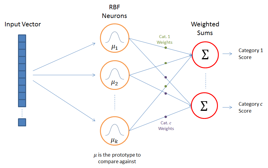
And here’s what it looks like for function approximation:

The difference in training is pretty straightforward. Each training example should have a set of input attributes, as well as the desired output value.

For classification, the desired output was either 0 or 1. ‘1’ if the training example belonged to the same category as the output node, and 0 otherwise. Training then optimizes the weights to get the output as close as possible to these desired value.

For function approximation the desired output is just the output value associated with the training example. In our housing price example, the training data would be examples of homes that have previously been sold, and the price they were sold at. So the desired output value is just the actual sell price.

RBF Neuron Width

Recall that each RBF neuron applies a Gaussian to the input. We all know from studying bell curves that an important parameter of the Gaussian is the standard deviation–it controls how wide the bell is. That same parameter exists here with our RBF neurons, you’d probably just interperet it a little differently. It still controls the width of the Gaussian, which means it determines how much of the input space the RBF neuron will respond to.

For RBFNs, instead of talking about the standard deviation (‘sigma’) directly, we use the related value ‘beta’:

Here are some examples of how different beta values affect the width of the Gaussian.

For classification, there are some good techniques for “learning” a good width value to use for each RBF neuron. The same technique doesn’t seem to work as well for function approximation, however, and it seems that a more primitive approach is often used. The width parameter is user provided, and is the same for every RBF neuron.

This means that the parameter is generally selected through experimentation. You can try different values, and then see how well the trained network performs on some hold-out validation examples. It’s important to optimize the parameter using hold-out data, because otherwise it’s too easy to for an RBFN to overfit the training data and generalize poorly.

Normalizing Neuron Activations

The final difference with function approximation RBFNs is that normalizing the RBF neuron activations often improves the accuracy of the approximation.

What is meant by normalization here? Every RBF neuron is going to produce an “activation value” between 0 and 1. To normalize the output of the RBFN, we simply divide the output by the sum of all of the RBF neuron activations.

Here is the equation for an RBFN without normalization:

To add normalization, we just divide by the sum of all of the activation values:

I’ve tried to come up with a good rationalization for why normalization improves things, but so far I’ve come up short.

There may be some insight gained from looking at Gaussian Kernel Regression… Gaussian Kernel Regression is just a particular case of a normalized RBFN that doesn’t require training. You create an RBF neuron for every single training example, and the output weights are just set equal to the output values of the training examples. In this case, the model is just calculating a distance-weighted average of the training example output values. It is fairly intuitive why normalization produces good results in this case. The intuition doesn’t quite apply to a trained RBFN, though, because the output weights are learned through optimization, and don’t necessarily correspond to the desired output values.

Matlab Code

RBFN for function approximation example code.

I’ve added the function approximation code to my existing RBFN classification example. For function approximation, you can run ‘runRBFNFuncApproxExample.m’. It uses many of the same functions as the classification RBFN, except that you train the RBFN with ‘trainFuncApproxRBFN.m’ and evaluate it with ‘evaluateFuncApproxRBFN.m’.