Latent Semantic Analysis (LSA) for Text Classification Tutorial

25 Mar 2016

In this post I'll provide a tutorial of Latent Semantic Analysis as well as some Python example code that shows the technique in action.

Why LSA?

Latent Semantic Analysis is a technique for creating a vector representation of a document. Having a vector representation of a document gives you a way to compare documents for their similarity by calculating the distance between the vectors. This in turn means you can do handy things like classifying documents to determine which of a set of known topics they most likely belong to.

Classification implies you have some known topics that you want to group documents into, and that you have some labelled training data. If you want to identify natural groupings of the documents without any labelled data, you can use clustering (see my post on clustering with LSA here).

tf-idf

The first step in LSA is actually a separate algorithm that you may already be familiar with. It’s called term frequency-inverse document frequency, or tf-idf for short.

tf-idf is pretty simple and I won’t go into it here, but the gist of it is that each position in the vector corresponds to a different word, and you represent a document by counting the number of times each word appears. Additionally, you normalize each of the word counts by the frequency of that word in your overall document collection, to give less frequent terms more weight.

There’s some thorough material on tf-idf in the Stanford NLP course available on YouTube here–specifically, check out the lectures 19-1 to 19-7. Or if you prefer some (dense) reading, you can check out the tf-idf chapter of the Stanford NLP textbook here.

LSA

Latent Semantic Analysis takes tf-idf one step further.

Side note: "Latent Semantic Analysis (LSA)" and "Latent Semantic Indexing (LSI)" are the same thing, with the latter name being used sometimes when referring specifically to indexing a collection of documents for search ("Information Retrieval").

LSA is quite simple, you just use SVD to perform dimensionality reduction on the tf-idf vectors–that’s really all there is to it!

If you're unfamiliar with dimensionality reduction, this topic was covered well in the Machine Learning course on Coursera. You can also find the lecture on YouTube here.

You might think to do this even if you had never heard of “LSA”–the tf-idf vectors tend to be long and unwieldy since they have one component for every word in the vocabulary. For instance, in my example Python code, these vectors have 10,000 components. So dimensionality reduction makes them more manageable for further operations like clustering or classification.

However, the SVD step does more than just reduce the computational load–you are trading a large number of features for a smaller set of better features.

What makes the LSA features better? I think the challenging thing with interpereting LSA is that you can talk about the behaviors that it is theoretically capable of doing, but ultimately what it does is dictated by the mathematical operations of SVD.

For example. A linear combination of terms is capable of handling pysnonyms: if you assign the words “car” and “automobile” the same weight, then they will contribute equally to the resulting LSA component, and it doesn’t matter which term the author uses.

You can find a little more discussion of the interpretation of LSA here. Also, the Python code associated with this post performs some inspection of the LSA results to try to gain some intuition.

LSA Python Code

Note: If you're less interested in learning LSA and just want to use it, you might consider checking out the nice gensim package in Python, it's built specifically for working with topic-modeling techniques like LSA.

I implemented an example of document classification with LSA in Python using scikit-learn. My code is available on GitHub, you can either visit the project page here, or download the source directly.

scikit-learn already includes a document classification example. However, that example uses plain tf-idf rather than LSA, and is geared towards demonstrating batch training on large datasets. Still, I borrowed code from that example for things like retrieving the Reuters dataset.

I wanted to put the emphasis on the feature extraction and not the classifier, so I used simple k-nn classification with k = 5 (majority wins).

Inspecting LSA

A little background on this Reuters dataset. These are news articles that were sent over the Reuters newswire in 1987. The dataset contains about 100 categories such as ‘mergers and acquisitions’, ‘interset rates’, ‘wheat’, ‘silver’ etc. Articles can be assigned multiple categories. The distribution of articles among categories is highly non-uniform; for example, the ‘earnings’ category contains 2,709 articles. And 75 of the categories contain less than 10 docs each!

Armed with that background, let’s see what LSA is learning from the dataset.

You can look at component 0 of the SVD matrix, and look at the terms which are given the highest weight by this component.

Top 10 Terms in Component 0

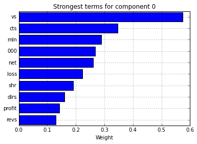
These terms are all very common to articles in the “earnings” category, which seem to be very terse. Here are some of the abbreviations used:

vs - “versus”
cts - “cents”
mln - “million”
shr - “share”
dlrs - “dollars”

Here’s an example earnings article from the dataset to give you some context:

COBANCO INC CBCO> YEAR NET

Shr 34 cts vs 1.19 dlrs Net 807,000 vs 2,858,000 Assets 510.2 mln vs 479.7 mln Deposits 472.3 mln vs 440.3 mln Loans 299.2 mln vs 327.2 mln Note: 4th qtr not available. Year includes 1985 extraordinary gain from tax carry forward of 132,000 dlrs, or five cts per shr. Reuter