Word2Vec Tutorial Part 2 - Negative Sampling

In part 2 of the word2vec tutorial (here’s part 1), I’ll cover a few additional modifications to the basic skip-gram model which are important for actually making it feasible to train.

When you read the tutorial on the skip-gram model for Word2Vec, you may have noticed something–it’s a huge neural network!

In the example I gave, we had word vectors with 300 components, and a vocabulary of 10,000 words. Recall that the neural network had two weight matrices–a hidden layer and output layer. Both of these layers would have a weight matrix with 300 x 10,000 = 3 million weights each!

Running gradient descent on a neural network that large is going to be slow. And to make matters worse, you need a huge amount of training data in order to tune that many weights and avoid over-fitting. millions of weights times billions of training samples means that training this model is going to be a beast.

The authors of Word2Vec addressed these issues in their second paper with the following two innovations:

1. Subsampling frequent words to decrease the number of training examples.
2. Modifying the optimization objective with a technique they called “Negative Sampling”, which causes each training sample to update only a small percentage of the model’s weights.

It’s worth noting that subsampling frequent words and applying Negative Sampling not only reduced the compute burden of the training process, but also improved the quality of their resulting word vectors as well.

Subsampling Frequent Words

In part 1 of this tutorial, I showed how training samples were created from the source text, but I’ll repeat it here. The below example shows some of the training samples (word pairs) we would take from the sentence “The quick brown fox jumps over the lazy dog.” I’ve used a small window size of 2 just for the example. The word highlighted in blue is the input word.

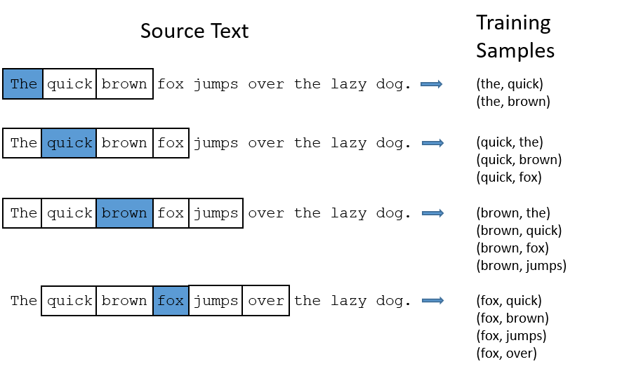
There are two “problems” with common words like “the”:

1. When looking at word pairs, (“fox”, “the”) doesn’t tell us much about the meaning of “fox”. “the” appears in the context of pretty much every word.
2. We will have many more samples of (“the”, …) than we need to learn a good vector for “the”.

Word2Vec implements a “subsampling” scheme to address this. For each word we encounter in our training text, there is a chance that we will effectively delete it from the text. The probability that we cut the word is related to the word’s frequency.

If we have a window size of 10, and we remove a specific instance of “the” from our text:

1. As we train on the remaining words, “the” will not appear in any of their context windows.
2. We’ll have 10 fewer training samples where “the” is the input word.

Note how these two effects help address the two problems stated above.

Sampling rate

The word2vec C code implements an equation for calculating a probability with which to keep a given word in the vocabulary.

\( w_i \) is the word, \( z(w_i) \) is the fraction of the total words in the corpus that are that word. For example, if the word “peanut” occurs 1,000 times in a 1 billion word corpus, then z(‘peanut’) = 1E-6.

There is also a parameter in the code named ‘sample’ which controls how much subsampling occurs, and the default value is 0.001. Smaller values of ‘sample’ mean words are less likely to be kept.

\( P(w_i) \) is the probability of keeping the word:

You can plot this quickly in Google to see the shape.

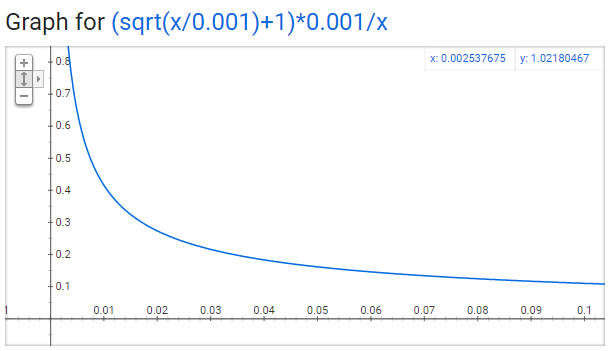
No single word should be a very large percentage of the corpus, so we want to look at pretty small values on the x-axis.

Here are some interesting points in this function (again this is using the default sample value of 0.001).

• \( P(w_i) = 1.0 \) (100% chance of being kept) when \( z(w_i) <= 0.0026 \).
  • This means that only words which represent more than 0.26% of the total words will be subsampled.
• \( P(w_i) = 0.5 \) (50% chance of being kept) when \( z(w_i) = 0.00746 \).
• \( P(w_i) = 0.033 \) (3.3% chance of being kept) when \( z(w_i) = 1.0 \).
  • That is, if the corpus consisted entirely of word \( w_i \), which of course is ridiculous.

Negative Sampling

Training a neural network means taking a training example and adjusting all of the neuron weights slightly so that it predicts that training sample more accurately. In other words, each training sample will tweak all of the weights in the neural network.

As we discussed above, the size of our word vocabulary means that our skip-gram neural network has a tremendous number of weights, all of which would be updated slightly by every one of our billions of training samples!

Negative sampling addresses this by having each training sample only modify a small percentage of the weights, rather than all of them. Here’s how it works.

When training the network on the word pair (“fox”, “quick”), recall that the “label” or “correct output” of the network is a one-hot vector. That is, for the output neuron corresponding to “quick” to output a 1, and for all of the other thousands of output neurons to output a 0.

With negative sampling, we are instead going to randomly select just a small number of “negative” words (let’s say 5) to update the weights for. (In this context, a “negative” word is one for which we want the network to output a 0 for). We will also still update the weights for our “positive” word (which is the word “quick” in our current example).

Recall that the output layer of our model has a weight matrix that’s 300 x 10,000. So we will just be updating the weights for our positive word (“quick”), plus the weights for 5 other words that we want to output 0. That’s a total of 6 output neurons, and 1,800 weight values total. That’s only 0.06% of the 3M weights in the output layer!

In the hidden layer, only the weights for the input word are updated (this is true whether you’re using Negative Sampling or not).

Selecting Negative Samples

The “negative samples” (that is, the 5 output words that we’ll train to output 0) are selected using a “unigram distribution”, where more frequent words are more likely to be selected as negative samples.

For instance, suppose you had your entire training corpus as a list of words, and you chose your 5 negative samples by picking randomly from the list. In this case, the probability for picking the word “couch” would be equal to the number of times “couch” appears in the corpus, divided the total number of word occus in the corpus. This is expressed by the following equation:

The authors state in their paper that they tried a number of variations on this equation, and the one which performed best was to raise the word counts to the 3/4 power:

If you play with some sample values, you’ll find that, compared to the simpler equation, this one has the tendency to increase the probability for less frequent words and decrease the probability for more frequent words.

The way this selection is implemented in the C code is interesting. They have a large array with 100M elements (which they refer to as the unigram table). They fill this table with the index of each word in the vocabulary multiple times, and the number of times a word’s index appears in the table is given by \( P(w_i) \) * table_size. Then, to actually select a negative sample, you just generate a random integer between 0 and 100M, and use the word at that index in the table. Since the higher probability words occur more times in the table, you’re more likely to pick those.

Word Pairs and “Phrases”

The second word2vec paper also includes one more innovation worth discussing. The authors pointed out that a word pair like “Boston Globe” (a newspaper) has a much different meaning than the individual words “Boston” and “Globe”. So it makes sense to treat “Boston Globe”, wherever it occurs in the text, as a single word with its own word vector representation.

You can see the results in their published model, which was trained on 100 billion words from a Google News dataset. The addition of phrases to the model swelled the vocabulary size to 3 million words!

If you’re interested in their resulting vocabulary, I poked around it a bit and published a post on it here. You can also just browse their vocabulary here.

Phrase detection is covered in the “Learning Phrases” section of their paper. They shared their implementation in word2phrase.c–I’ve shared a commented (but otherwise unaltered) copy of this code here.

I don’t think their phrase detection approach is a key contribution of their paper, but I’ll share a little about it anyway since it’s pretty straightforward.

Each pass of their tool only looks at combinations of 2 words, but you can run it multiple times to get longer phrases. So, the first pass will pick up the phrase “New_York”, and then running it again will pick up “New_York_City” as a combination of “New_York” and “City”.

The tool counts the number of times each combination of two words appears in the training text, and then these counts are used in an equation to determine which word combinations to turn into phrases. The equation is designed to make phrases out of words which occur together often relative to the number of individual occurrences. It also favors phrases made of infrequent words in order to avoid making phrases out of common words like “and the” or “this is”.

You can see more details about their equation in my code comments here.

Other Resources

If you’re familiar with C, I’ve published an extensively commented (but otherwise unaltered) version of the original word2vec C code here.

Also, did you know that the word2vec model can also be applied to non-text data for recommender systems and ad targeting? Instead of learning vectors from a sequence of words, you can learn vectors from a sequence of user actions. Read more about this in my new post here.

eBook & Example Code

I think word2vec is a fascinating (and powerful!) algorithm–great work on making it this far in understanding it!

Maybe you still have some questions, though…

• Are you looking for a deeper explanation of how the model weights are updated?
• Would you like to know more about the technical and practical differences between the Skip-gram and Continuous Bag of Words (CBOW) versions of word2vec?
• Did you know that Mikolov, the main author of word2vec, has published further work on word2vec in the form of the fastText library from Facebook?
• Want to see all of the core word2vec components implemented from scratch in Python?

You’ll find all of the above content in my eBook The Inner Workings of word2vec. Give it a look, I think you’ll find it really valuable!

Cite

McCormick, C. (2017, January 11). Word2Vec Tutorial Part 2 - Negative Sampling. Retrieved from http://www.mccormickml.com