Matrix Operations in NumPy vs. Matlab

If your first foray into Machine Learning was with Andrew Ng’s popular Coursera course (which is where I started back in 2012!), then you learned the fundamentals of Machine Learning using example code in “Octave” (the open-source version of Matlab). Octave is great for expressing linear algebra operations cleanly, and (as I hear it) for being easier for non-programmers to get going with.

It’s also likely that you have since switched from Octave to Python. Coding in Python obviously means learning a whole new programming language, with many important differences, but those aren’t the subject of this post. Instead, I wanted to highlight some false assumptions that you may have brought with you from Matlab about how vector and matrix operations should work.

Side Note: The NumPy documentation has a very nice “quick reference” type guide on migrating from Matlab to NumPy here.

Turns out ndarray ≠ matrix

Once you have the basics of Python down, you’ll find that, in the machine learning field, we use NumPy ndarray to store our matrix and vector data. NumPy arrays behave very similarly to variables in Matlab–for instance, they both support very similar syntax for making selections within a matrix. This is great, and it makes the transition to Python a lot easier.

Based on these similarities, you’ll be tempted to think of the ndarray as generally equivalent to a Matlab matrix–I certainly did. But they’re not! They have some fundamental differences, and these differences are eventually going to trip you up if you’re not made aware of them.

In fact, did you know that NumPy actually has a separate class named numpy.matrix? Probably not–it’s not what the Python community typically uses. The existence of this separate matrix class should be a red flag–why would we need a separate matrix class if matrices are just 2D ndarrays?

Here are the two big differences.

1. If you have two matrices \( A \) and \( B \) both stored as numpy.ndarrays, then you’d probably think that running C = A * B performs matrix multiplication… but it doesn’t. The below table illustrates this with a matrix-vector multiplication example.

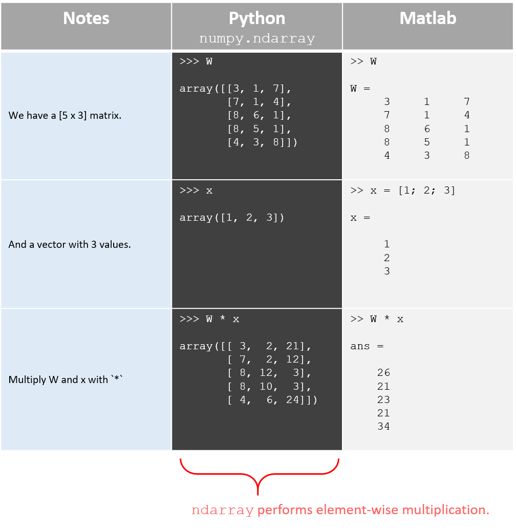
1. With numpy.ndarray, vectors tend to end up as 1-dimensional, meaning numpy doesn’t naturally distinguish between a row vector and a column vector.

Don’t use numpy.matrix

Before we explore these further, you should know that using numpy.matrix instead of numpy.ndarray will actually resolve both of these issues. The matrix class is designed to behave like matrix variables in Matlab. Using * does perform matrix multiplication, and the matrix type is always two dimensional, whether it’s storing a matrix or a vector, just like in Matlab.

However, don’t actually do this! The community (and libraries) don’t use numpy.matrix in practice (they even plan to deprecate it!). Using numpy.matrix will probably just get us into trouble in the long run, so I think we’re better off adjusting our thinking instead to using ndarray.

In the rest of the post we’ll do just that.

Issue #1: ndarray operations are element-wise

I think there’s a good reason that numpy.ndarray uses the term “array”. “Array” is a computer science term–in Python we call these “lists”, but in more formal languages like C or Java we have “arrays”.

If you’re teaching a software engineer the basics of machine learning, a good way to explain what a vector is, is that’s it’s “just an array of floating point values”.

So an array is a computer science concept, and not a linear algebra one.

If you’re NOT working in the context of Linear Algebra or Machine Learning, then interpreting “a * b” as an element-wise multiplication seems perflectly reasonable to me. The linear algebra interpretation is really the more bizarre one.

The solution is simple–stay away from the *, and just call the numpy.dot function.

import numpy as np

# Define matrix W with 5 rows and 3 columns.
W = np.asarray([[3, 1, 7], 
                [7, 1, 4],
                [8, 6, 1],
                [8, 5, 1],
                [4, 3, 8]], dtype='int')

# Define vector x with length 3.
x = np.asarray([1, 2, 3], dtype='int')

# `*` performs element-wise multiplication.
print(W * x)
print('')

# `np.dot` performs matrix-vector multiplication.
print(np.dot(W, x))

Outputs:

[[ 3  2 21]
 [ 7  2 12]
 [ 8 12  3]
 [ 8 10  3]
 [ 4  6 24]]

[26 21 23 21 34]

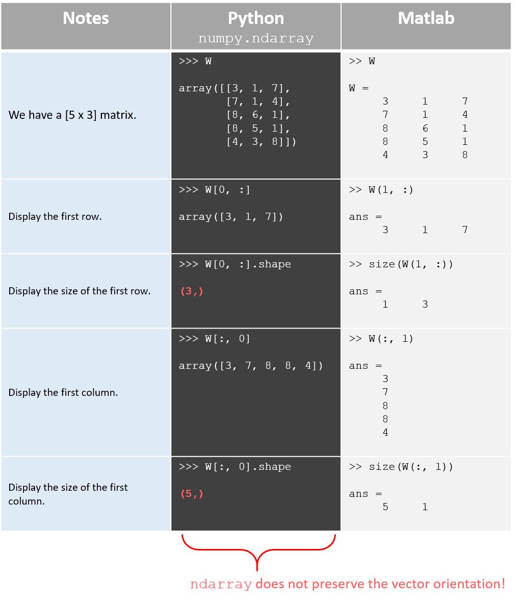
Issue #2: ndarray treats vectors as 1-dimensional

This difference has probably caused me the most grief.

In Matlab (and in numpy.matrix), a vector is a 2-dimensional object–it’s either a column vector (e.g., [5 x 1]) or a row vector (e.g., [1 x 5]).

In a NumPy ndarray, vectors tend to end up as 1-dimensional arrays.

Having only one dimension means that the vector has a length, but not an orientation (row vector vs. column vector). Check out the simple example below. The array shape is (5,).

Note: The syntax (5,) is kind of funky! But it’s just how Python represents a tuple with only one value.

import numpy as np

# Create an ndarray from a python list.
x = np.asarray([1, 2, 3, 4, 5])

# Print out its shape and contents.
print('Type:  ', type(x))
print('Shape: ', x.shape)
print('Values:', x)

Type:   <class 'numpy.ndarray'>
Shape:  (5,)
Values: [1 2 3 4 5]

Why would vector orientation matter?

The distinction between a row vector and a column vector is important in linear algebra, because if you have a matrix \( W \) that’s [5 x 3] and a column vector \( x \) that’s [5 x 1], then there are restrictions on how they can legally be multiplied together:

• \( xW \) - Not Valid
  • [5 x 1] * [5 x 3] = Error!
• \( Wx \) - Not Valid
  • [5 x 3] * [5 x 1] = Error!
• \( x’W \) - Valid
  • [1 x 5] * [5 x 3] = [1 x 3]
• \( W’x \) - Valid
  • [3 x 5] * [5 x 1] = [3 x 1]

Note that the output vectors of the last two (the two valid operations) not only have different orientations but also contain different values.

When implementing an algorithm in code based on its equation, I find the matrix and vector dimensions very helpful both for interpreting the equation and for ensuring that I am coding it correctly. I typically print out the dimensions of my matrices as a sanity check.

With the above definitions of x and W, if I try to write x * W in Matlab, then there’s clearly something wrong–I’m misinterpreting the equation somehow. Matlab will help make me aware of this by throwing an error that the dimensions don’t align.

NumPy, however, will simply assume that x is a row vector, and that np.dot(x, W) is valid.

import numpy as np

# Create a matrix X with 5 rows and 3 columns [5 x 3]
X = np.random.randint(low=0, high=10, size=(5, 3))

# Create a matrix W with 5 rows and 10 columns [5 x 10]
W = np.random.randint(low=0, high=10, size=(5,10))

# Select `x` as column 0 from X.
# In Matlab, this would have shape [5 x 1]
x = X[:, 0]

print('x:', x, '    x.shape:', x.shape, '\n')

# Multiply x with W.
# It should be illegal to multiply a [5 x 1] vector against a [5 x 10] matrix--
# the dimensions don't align. But because the orientation of `x` has 
# been dropped, NumPy assumes that you know what you're doing and that `x`
# is really a row vector with shape [1 x 5].
z = np.dot(x, W)

print('z:', z, '    z.shape', z.shape)

Outputs:

x: [2 7 2 1 0]     x.shape: (5,) 

z: [86 31 68 31 58 39 73 45 50 23]     z.shape (10,)

The solution

Option A: Reshape the ndarray vectors to 2D

If it bothers you so much, Chris, then why not simply call the reshape function on the vectors in NumPy to force them to have two dimensions?

This is a possibility, but it creates a couple new pitfalls that you’d need to be careful of. Plus, it leads to some rather funky syntax.

Here are the two problems with this approach:

(1) When you slice a vector from a matrix, the ndarray class drops any unneccessary dimensions. Again–this makes more sense when you’re thinking in terms of the computer science “array” concept and not the “matrix” concept. To combat this, you need to put the vector’s index inside square brackets, as if it were a list of multiple indeces that you wanted to select.

# Create a matrix with shape [5 x 3]
X_train = np.random.randint(low=0, high=10, size=(5, 3))

# Returns a 1D vector of length 3.
x = X_train[0, :]

# Returns a 2D row vector with shape [1 x 3]
x = X_train[[0], :]

(2) When you want to access a single value from 2D row vector, you must specify both dimensions.

# `x` is a 2D row vector with shape [1 x 3].
x = X_train[[0], :]

# `x[0]` returns an ndarray of length 3.
a = x[0]

# `x[0, 0]` returns the value at element 0 of the row vector.
a = x[0, 0]

Option B: Let it go!

I believe the simplest and best solution to the 1D vector problem, and the approach I plan to take, is simply to change my thinking away from 2D vectors.

I’ll just accept that vectors in numpy are 1D, and if I want to track their orientation explicitly, I’ll do that in my code comments, rather than by forcing the vector to 2-dimensions.

I went through a lot of headaches, confusion, and research in order to come to that simple conclusion–so I’m hoping you can learn from it and avoid my mistakes!