Domain-Specific BERT Models

22 Jun 2020

If your text data is domain specific (e.g. legal, financial, academic, industry-specific) or otherwise different from the “standard” text corpus used to train BERT and other langauge models you might want to consider either continuing to train BERT with some of your text data or looking for a domain-specific language model.

Faced with the issue mentioned above, a number of researchers have created their own domain-specific language models. These models are created by training the BERT architecture from scratch on a domain-specific corpus rather than the general purpose English text corpus used to train the original BERT model. This leads to a model with vocabulary and word embeddings better suited than the original BERT model to domain-specific NLP problems. Some examples include:

SciBERT (biomedical and computer science literature corpus)
FinBERT (financial services corpus)
BioBERT (biomedical literature corpus)
ClinicalBERT (clinical notes corpus)
mBERT (corpora from multiple languages)
patentBERT (patent corpus)

In this tutorial, we will:

Show you how to find domain-specific BERT models and import them using the transformers library in PyTorch.
Explore SciBERT and compare it’s vocabulary and embeddings to those in the original BERT.

Here is the Colab Notebook version of this post (it’s identical to the blog post).

by Chris McCormick and Nick Ryan

Contents
- 1.1 Why not do my own pre-training?
2. Using a Community-Submitted Model
- 2.1. Library of Models
- 2.2. Example Code for Importing
3. Comparing SciBERT and BERT
- 3.1. Comparing Vocabularies
  - Vocab Dump
  - Numbers and Symbols
- 3.2. Comparing Embeddings
Appendix: BioBERT vs. SciBERT

1.1 Why not do my own pre-training?

If you think your text is too domain-specific for the generic BERT, your first thought might be to train BERT from scratch on your own dataset. (Just to be clear: BERT was “Pre-Trained” by Google, and we download and “Fine-Tune” Google’s pre-trained model on our own data. When I say “train BERT from scratch”, I mean specifically re-doing BERT’s pre-training).

Chances are you won’t be able to pre-train BERT on your own dataset, though, for the following reasons.

1. Pre-training BERT requires a huge corpus

BERT-base is a 12-layer neural network with roughly 110 million weights. This enormous size is key to BERT’s impressive performance. To train such a complex model, though, (and expect it to work) requires an enormous dataset, on the order of 1B words. Wikipedia is a suitable corpus, for example, with its ~10 million articles. For the majority of applications I assume you won’t have a dataset with that many documents.

2. Huge Model + Huge Corpus = Lots of GPUs

Pre-Training BERT is expensive. The cost of pre-training is a whole subject of discussion, and there’s been a lot of work done on bringing the cost down, but a single pre-training experiment could easily cost you thousands of dollars in GPU or TPU time.

That’s why these domain-specific pre-trained models are so interesting. Other organizations have footed the bill to produce and share these models which, while not pre-trained on your specific dataset, may at least be much closer to yours than “generic” BERT.

2. Using a Community-Submitted Model

2.1. Library of Models

The list of domain-specific models in the introduction are just a few examples of the models that have been created, so it’s worth looking for and trying out an open-source model in your domain if it exists.

Fortunately, many of the popular models (and many unpopular ones!) have been uploaded by the community into the transformers library; you can browse the full list of models at: https://huggingface.co/models

’’

It’s not very easy to browse, however–there are currently over 1,700 models shared!

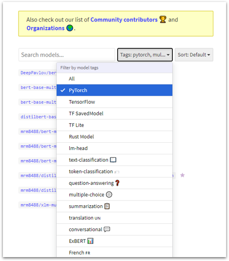
If you know the name of the model you’re looking for, you can search this list by keyword. But if you’re looking for a specific type of model, there is a “tags” filter option next to the search bar.

For example, if you filter for “Multilingual” and “Pytorch”, it narrows it done to just 10 models.

Side Note: If you skim the full list you’ll see that roughly 1,000 of the current models are variants of a single machine translation model from “Helsinki NLP”. There is a different variant for every pair of languages. For example, English to French: Helsinki-NLP/opus-mt-en-fr

For this Notebook, we’ll use SciBERT, a popular BERT variant trained primarily on biomedical literature.

Each model has its own page in the huggingface library where you can learn a little more about it: https://huggingface.co/allenai/scibert_scivocab_uncased

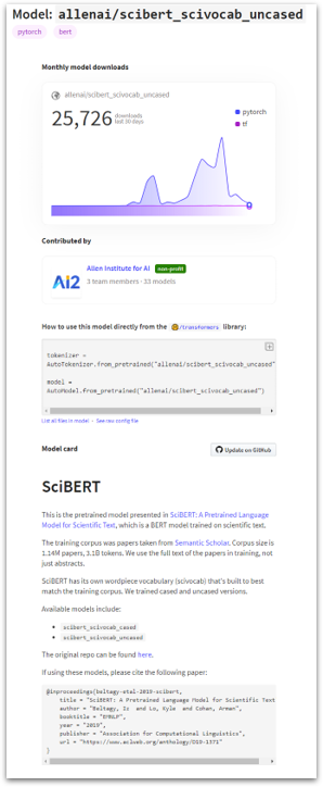
Here are some highlights:

SciBERT was trained on scientific literature–1.14M papers.
- ~1/5th of the papers are from “the computer science domain”
- ~4/5th of the papers are from “the broad biomedical domain”.
SciBERT was created by the Allen Institute of AI (a highly respected group in NLP, if you’re unfamiliar).
Their paper was first submitted to arXiv in March, 2019 here. They uploaded their implementation to GitHub here around the same time.

2.2. Example Code for Importing

If you’re interested in a BERT variant from the community models in the transformers library, importing can be incredibly simple–you just supply the name of the model as it appears in the library page.

First, we’ll need to install the transformers library.

!pip install transformers

The transformers library includes classes for different model architectures (e.g., BertModel, AlbertModel, RobertaModel, …). With whatever model you’re using, it needs to be loaded with the correct class (based on its architecture), which may not be immediately apparent.

Luckily, the transformers library has a solution for this, demonstrated in the following cell. These “Auto” classes will choose the correct architecture for you!

That’s a nice feature, but I’d still prefer to know what I’m working with, so I’m printing out the class names (which show that SciBERT uses the original BERT classes).

from transformers import AutoTokenizer, AutoModel
import torch

scibert_tokenizer = AutoTokenizer.from_pretrained("allenai/scibert_scivocab_uncased")
scibert_model = AutoModel.from_pretrained("allenai/scibert_scivocab_uncased")

print('scibert_tokenizer is type:', type(scibert_tokenizer))
print('    scibert_model is type:', type(scibert_model))

scibert_tokenizer is type: <class 'transformers.tokenization_bert.BertTokenizer'>
    scibert_model is type: <class 'transformers.modeling_bert.BertModel'>

3. Comparing SciBERT and BERT

3.1. Comparing Vocabularies

The most apparent difference between SciBERT and the original BERT should be the model’s vocabulary, since they were trained on such different corpuses.

Both tokenizers have a 30,000 word vocabulary that was automatically built based on the most frequently seen words and subword units in their respective corpuses.

The authors of SciBERT note:

“The resulting token overlap between [BERT vocabulary] and [SciBERT vocabulary] is 42%, illustrating a substantial difference in frequently used words between scientific and general domain texts.”

Let’s load the original BERT as well and do some of our own comparisons.

Side note: BERT used a “WordPiece” model for tokenization, whereas SciBERT employs a newer approach called “SentencePiece”, but the difference is mostly cosmetic. I cover SentencePiece in more detail in our ALBERT eBook.

from transformers import BertTokenizer, BertModel

bert_tokenizer = BertTokenizer.from_pretrained('bert-base-uncased')
bert_model = BertModel.from_pretrained('bert-base-uncased')

Let’s apply both tokenizers to some biomedical text and see how they compare.

I took the below sentence from the 2001 paper Hydrogels for biomedical applications, which seems to be one of the most-cited papers in the field of biomedical applications (if I’m interpreting these Google Scholar results correctly).

text = "Hydrogels are hydrophilic polymer networks which may absorb from " \
       "10–20% (an arbitrary lower limit) up to thousands of times their " \
       "dry weight in water."

# Split the sentence into tokens, with both BERT and SciBERT.
bert_tokens = bert_tokenizer.tokenize(text)
scibert_tokens = scibert_tokenizer.tokenize(text)

# Pad out the scibert list to be the same length.
while len(scibert_tokens) < len(bert_tokens):
    scibert_tokens.append("")

# Label the columns.
print('{:<12} {:<12}'.format("BERT", "SciBERT"))
print('{:<12} {:<12}'.format("----", "-------"))

# Display the tokens.
for tup in zip(bert_tokens, scibert_tokens):
    print('{:<12} {:<12}'.format(tup[0], tup[1]))

BERT         SciBERT     
----         -------     
hydro        hydrogels   
##gel        are         
##s          hydrophilic 
are          polymer     
hydro        networks    
##phi        which       
##lic        may         
polymer      absorb      
networks     from        
which        10          
may          –           
absorb       20          
from         %           
10           (           
–            an          
20           arbitrary   
%            lower       
(            limit       
an           )           
arbitrary    up          
lower        to          
limit        thousands   
)            of          
up           times       
to           their       
thousands    dry         
of           weight      
times        in          
their        water       
dry          .           
weight                   
in                       
water                    
.                        

SciBERT apparently has embeddings for the words ‘hydrogels’ and ‘hydrophillic’, whereas BERT had to break these down into three subwords each. (Remember that the ‘##’ in a token is just a way to flag it as a subword that is not the first subword). Apparently BERT does have “polymer”, though!

I skimmed the paper and pulled out some other esoteric terms–check out the different numbers of tokens required by each model.

# Use pandas just for table formatting.
import pandas as pd

# Some strange terms from the paper.
words = ['polymerization', 
         '2,2-azo-isobutyronitrile',
         'multifunctional crosslinkers'
         ]

# For each term...
for word in words:
    
    # Print it out
    print('\n\n', word, '\n')

    # Start a list of tokens for each model, with the first one being the model name.
    list_a = ["BERT:"]
    list_b = ["SciBERT:"]

    # Run both tokenizers.
    list_a.extend(bert_tokenizer.tokenize(word))
    list_b.extend(scibert_tokenizer.tokenize(word))

    # Pad the lists to the same length.
    while len(list_a) < len(list_b):
        list_a.append("")
    while len(list_b) < len(list_a):
        list_b.append("")

    # Wrap them in a DataFrame to display a pretty table.
    df = pd.DataFrame([list_a, list_b])
    
    display(df)

 polymerization

	0	1	2
0	BERT:	polymer	##ization
1	SciBERT:	polymerization

 2,2-azo-isobutyronitrile

	0	1	2	3	4	5	6	7	8	9	10	11	12	13	14
0	BERT:	2	,	2	-	az	##o	-	iso	##bu	##ty	##ron	##it	##ril	##e
1	SciBERT:	2	,	2	-	az	##o	-	iso	##but	##yr	##onitrile

 multifunctional crosslinkers

	0	1	2	3	4	5	6	7
0	BERT:	multi	##fu	##nction	##al	cross	##link	##ers
1	SciBERT:	multifunctional	cross	##link	##ers

The fact that SciBERT is able to represent all of these terms in fewer tokens seems like a good sign!

Vocab Dump

It can be pretty interesting just to dump the full vocabulary of a model into a text file and skim it to see what stands out.

This cell will write out SciBERT’s vocab to ‘vocabulary.txt’, which you can open in Colab by going to the ‘Files’ tab in the pane on the left and double clicking the .txt file.

with open("vocabulary.txt", 'w') as f:
    
    # For each token in SciBERT's vocabulary...
    for token in scibert_tokenizer.vocab.keys():
        
        # Write it out, one per line.
        f.write(token + '\n')

You’ll see that roughly the first 100 tokens are reserved, and then it looks like the rest of the vocabulary is sorted by frequency… The first actual tokens are:

t, a, ##in, ##he, ##re, ##on, the, s, ##ti

Because the tokenizer breaks down “unknown” words into subtokens, it makes sense that some individual characters and subwords would be higher in frequency even than the most common words like “the”.

Numbers and Symbols

There seem to be a lot of number-related tokens in SciBERT–you see them constantly as you scroll through the vocabulary. Here are some examples:

"##.2%)" in scibert_tokenizer.vocab

True

"0.36" in scibert_tokenizer.vocab

True

In the below loops, we’ll tally up the number of tokens which include a digit, and show a random sample of these tokens. We’ll do this for both SciBERT and BERT for comparison.

import random

# ======== BERT ========
bert_examples = []

count = 0

# For each token in the vocab...
for token in bert_tokenizer.vocab:
    
    # If there's a digit in the token...
    # (But don't count those reserved tokens, e.g. "[unused59]")
    if any(i.isdigit() for i in token) and not ('unused' in token):
        # Count it.
        count += 1

        # Keep ~1% as examples to print.
        if random.randint(0, 100) == 1:
            bert_examples.append(token)

# Calculate the count as a percentage of the total vocab.
prcnt = float(count) / len(bert_tokenizer.vocab)

# Print the result.
print('In BERT:    {:>5,} tokens ({:.2%}) include a digit.'.format(count, prcnt))

# ======== SciBERT ========
scibert_examples = []
count = 0

# For each token in the vocab...
for token in scibert_tokenizer.vocab:

    # If there's a digit in the token...
    # (But don't count those reserved tokens, e.g. "[unused59]")
    if any(i.isdigit() for i in token) and not ('unused' in token):
        # Count it.
        count += 1

        # Keep ~1% as examples to print.
        if random.randint(0, 100) == 1:
            scibert_examples.append(token)
   

# Calculate the count as a percentage of the total vocab.
prcnt = float(count) / len(scibert_tokenizer.vocab)

# Print the result.
print('In SciBERT: {:>5,} tokens ({:.2%}) include a digit.'.format(count, prcnt))

print('')
print('Examples from BERT:', bert_examples)
print('Examples from SciBERT:', scibert_examples)

In BERT:    1,109 tokens (3.63%) include a digit.
In SciBERT: 3,345 tokens (10.76%) include a digit.

Examples from BERT: ['5', '2002', '1971', '1961', 'm²', '355']
Examples from SciBERT: ['3.', '(1)', '##8).', '##0).', '##9–', '53', '16,', '[10].', '(1999)', '194', '[3],', '##1,2', '15%', '##:12', '(2001).', '##(4):', '##103', '##27,', '10.1002/', '##21)', '100.', '##(1+', '13).', '241', '(54', '##2)2']

So it looks like:

SciBERT has about 3x as many tokens with digits.
BERT’s tokens are whole integers, and many look like they could be dates. (In another Notebook, I showed that BERT contains 384 of the integers in the range 1600 - 2021).
SciBERT’s number tokens are much more diverse. They are often subwords, and many include decimal places or other symbols like % or (.

Random – check out token 17740!:

⎝

Looks like something is stuck to your monitor! o_O

3.2. Comparing Embeddings

Semantic Similarity on Scientific Text

To create a simple demonstration of SciBERT’s value, Nick and I figured we could create a semantic similarity example where we show that SciBERT is better able to recognize similarities and differences within some scientific text than generic BERT.

We implemented this idea, but the examples we tried don’t appear to show SciBERT as being better!

We thought our code and results are interesting to share all the same.

Also, while our simple example didn’t succeed, note that the authors of SciBERT rigorously demonstrate its value over the original BERT by reporting results on a number of different NLP benchmarks that are focused specifically on scientific text. You can find the results in their paper here.

Our Approach

In our semantic similarity task, we have three pieces of text–call them “query”, “A”, and “B”, that are all on scientific topics. We pick these such that the query text is always more similar to A than to B.

Here’s an example:

query: “Mitochondria (mitochondrion, singular) are membrane-bound cell organelles.”
A: “These powerhouses of the cell produce adenosine triphosphate (ATP).”
B: “Ribosomes contain RNA and are responsible for synthesizing the proteins needed for many cellular functions.”

query and A are both about mitochondria, whereas B is about ribosomes. However, to recognize the similarity between query and A, you would need to know that mitochondria are responsible for producing ATP.

Our intuition was that SciBERT, being trained on biomedical text, would better distinguish the similarities than BERT.

Interpreting Cosine Similarities

When comparing two different models for semantic similarity, it’s best to look at how well they rank the similarities, and not to compare the specific cosine similarity values across the two models.

It’s for this reason that we’ve structured our example as “is query more similar to A or to B?”

Embedding Functions

In order to try out different examples, we’ve defined a get_embedding function below. It takes the average of the embeddings from the second-to-last layer of the model to use as a sentence embedding.

get_embedding also supports calculating an embedding for a specific word or sequence of words within the sentence.

To locate the indeces of the tokens for these words, we’ve also defined the get_word_indeces helper function below.

To calculate the word embedding, we again take the average of its token embeddings from the second-to-last layer of the model.

get_word_indeces

import numpy as np

def get_word_indeces(tokenizer, text, word):
    '''
    Determines the index or indeces of the tokens corresponding to `word`
    within `text`. `word` can consist of multiple words, e.g., "cell biology".
    
    Determining the indeces is tricky because words can be broken into multiple
    tokens. I've solved this with a rather roundabout approach--I replace `word`
    with the correct number of `[MASK]` tokens, and then find these in the 
    tokenized result. 
    '''
    # Tokenize the 'word'--it may be broken into multiple tokens or subwords.
    word_tokens = tokenizer.tokenize(word)

    # Create a sequence of `[MASK]` tokens to put in place of `word`.
    masks_str = ' '.join(['[MASK]']*len(word_tokens))

    # Replace the word with mask tokens.
    text_masked = text.replace(word, masks_str)

    # `encode` performs multiple functions:
    #   1. Tokenizes the text
    #   2. Maps the tokens to their IDs
    #   3. Adds the special [CLS] and [SEP] tokens.
    input_ids = tokenizer.encode(text_masked)

    # Use numpy's `where` function to find all indeces of the [MASK] token.
    mask_token_indeces = np.where(np.array(input_ids) == tokenizer.mask_token_id)[0]

    return mask_token_indeces

get_embedding

def get_embedding(b_model, b_tokenizer, text, word=''):
    '''
    Uses the provided model and tokenizer to produce an embedding for the
    provided `text`, and a "contextualized" embedding for `word`, if provided.
    '''

    # If a word is provided, figure out which tokens correspond to it.
    if not word == '':
        word_indeces = get_word_indeces(b_tokenizer, text, word)

    # Encode the text, adding the (required!) special tokens, and converting to
    # PyTorch tensors.
    encoded_dict = b_tokenizer.encode_plus(
                        text,                      # Sentence to encode.
                        add_special_tokens = True, # Add '[CLS]' and '[SEP]'
                        return_tensors = 'pt',     # Return pytorch tensors.
                )

    input_ids = encoded_dict['input_ids']
    
    b_model.eval()

    # Run the text through the model and get the hidden states.
    bert_outputs = b_model(input_ids)
    
    # Run the text through BERT, and collect all of the hidden states produced
    # from all 12 layers. 
    with torch.no_grad():

        outputs = b_model(input_ids)

        # Evaluating the model will return a different number of objects based on 
        # how it's  configured in the `from_pretrained` call earlier. In this case, 
        # becase we set `output_hidden_states = True`, the third item will be the 
        # hidden states from all layers. See the documentation for more details:
        # https://huggingface.co/transformers/model_doc/bert.html#bertmodel
        hidden_states = outputs[2]

    # `hidden_states` has shape [13 x 1 x <sentence length> x 768]

    # Select the embeddings from the second to last layer.
    # `token_vecs` is a tensor with shape [<sent length> x 768]
    token_vecs = hidden_states[-2][0]

    # Calculate the average of all token vectors.
    sentence_embedding = torch.mean(token_vecs, dim=0)

    # Convert to numpy array.
    sentence_embedding = sentence_embedding.detach().numpy()

    # If `word` was provided, compute an embedding for those tokens.
    if not word == '':
        # Take the average of the embeddings for the tokens in `word`.
        word_embedding = torch.mean(token_vecs[word_indeces], dim=0)

        # Convert to numpy array.
        word_embedding = word_embedding.detach().numpy()
    
        return (sentence_embedding, word_embedding)
    else:
        return sentence_embedding

Retrieve the models and tokenizers for both BERT and SciBERT

from transformers import BertModel, BertTokenizer

# Retrieve SciBERT.
scibert_model = BertModel.from_pretrained("allenai/scibert_scivocab_uncased",
                                  output_hidden_states=True)
scibert_tokenizer = BertTokenizer.from_pretrained("allenai/scibert_scivocab_uncased")

scibert_model.eval()

# Retrieve generic BERT.
bert_model = BertModel.from_pretrained('bert-base-uncased',
                                  output_hidden_states = True) 
bert_tokenizer = BertTokenizer.from_pretrained('bert-base-uncased')

bert_model.eval()

Test out the function.

text = "hydrogels are hydrophilic polymer networks which may absorb from 10–20% (an arbitrary lower limit) up to thousands of times their dry weight in water."
word = 'hydrogels'

# Get the embedding for the sentence, as well as an embedding for 'hydrogels'.
(sen_emb, word_emb) = get_embedding(scibert_model, scibert_tokenizer, text, word)

print('Embedding sizes:')
print(sen_emb.shape)
print(word_emb.shape)

Embedding sizes:
(768,)
(768,)

Here’s the code for calculating cosine similarity. We’ll test it by comparing the word embedding with the sentence embedding–not a very interesting comparison, but a good sanity check.

from scipy.spatial.distance import cosine

# Calculate the cosine similarity of the two embeddings.
sim = 1 - cosine(sen_emb, word_emb)

print('Cosine similarity: {:.2}'.format(sim))

Cosine similarity: 0.86

Sentence Comparison Examples

In this example, query and A are about biomedical “hydrogels”, and B is from astrophysics.

Both models make the correct distinction, but generic BERT seems to be better…

# Three sentences; query is more similar to A than B.
text_query = "Chemical hydrogels are commonly prepared in two different ways: ‘three-dimensional polymerization’ (Fig. 1), in which a hydrophilic monomer is polymerized in the presence of a polyfunctional cross-linking agent, or by direct cross-linking of water-soluble polymers (Fig. 2)."
text_A = "Hydrogels can be obtained by radiation technique in a few ways, including irradiation of solid polymer, monomer (in bulk or in solution), or aqueous solution of polymer."
text_B = "The observed cosmic shear auto-power spectrum receives an additional contribution due to shape noise from intrinsic galaxy ellipticities."

# Get embeddings for each.
emb_query = get_embedding(scibert_model, scibert_tokenizer, text_query)
emb_A = get_embedding(scibert_model, scibert_tokenizer, text_A)
emb_B = get_embedding(scibert_model, scibert_tokenizer, text_B)

# Compare query to A and B with cosine similarity.
sim_query_A = 1 - cosine(emb_query, emb_A)
sim_query_B = 1 - cosine(emb_query, emb_B)

print("'query' should be more similar to 'A' than to 'B'...\n")

print('SciBERT:')
print('  sim(query, A): {:.2}'.format(sim_query_A))
print('  sim(query, B): {:.2}'.format(sim_query_B))

# Repeat with BERT.
emb_query = get_embedding(bert_model, bert_tokenizer, text_query)
emb_A = get_embedding(bert_model, bert_tokenizer, text_A)
emb_B = get_embedding(bert_model, bert_tokenizer, text_B)

# Compare query to A and B with cosine similarity.
sim_query_A = 1 - cosine(emb_query, emb_A)
sim_query_B = 1 - cosine(emb_query, emb_B)

print('')
print('BERT:')
print('  sim(query, A): {:.2}'.format(sim_query_A))
print('  sim(query, B): {:.2}'.format(sim_query_B))

'query' should be more similar to 'A' than to 'B'...

SciBERT:
  sim(query, A): 0.96
  sim(query, B): 0.89

BERT:
  sim(query, A): 0.92
  sim(query, B): 0.65

In this example, query and A are both about mitochondria, while B is about ribosomes.

Neither model seems to recognize the distinction!

# Three sentences; query is more similar to A than B.
text_query = "Mitochondria (mitochondrion, singular) are membrane-bound cell organelles."
text_A = "These powerhouses of the cell produce adenosine triphosphate (ATP)." 
text_B = "Ribosomes contain RNA and are responsible for synthesizing the proteins needed for many cellular functions."
#text_B = "Molecular biology deals with the structure and function of the macromolecules (e.g. proteins and nucleic acids) essential to life." 

# Get embeddings for each.
emb_query = get_embedding(scibert_model, scibert_tokenizer, text_query)
emb_A = get_embedding(scibert_model, scibert_tokenizer, text_A)
emb_B = get_embedding(scibert_model, scibert_tokenizer, text_B)

# Compare query to A and B with cosine similarity.
sim_query_A = 1 - cosine(emb_query, emb_A)
sim_query_B = 1 - cosine(emb_query, emb_B)

print("'query' should be more similar to 'A' than to 'B'...\n")

print('SciBERT:')
print('  sim(query, A): {:.2}'.format(sim_query_A))
print('  sim(query, B): {:.2}'.format(sim_query_B))

# Repeat with BERT.
emb_query = get_embedding(bert_model, bert_tokenizer, text_query)
emb_A = get_embedding(bert_model, bert_tokenizer, text_A)
emb_B = get_embedding(bert_model, bert_tokenizer, text_B)

# Compare query to A and B with cosine similarity.
sim_query_A = 1 - cosine(emb_query, emb_A)
sim_query_B = 1 - cosine(emb_query, emb_B)

print('')
print('BERT:')
print('  sim(query, A): {:.2}'.format(sim_query_A))
print('  sim(query, B): {:.2}'.format(sim_query_B))

'query' should be more similar to 'A' than to 'B'...

SciBERT:
  sim(query, A): 0.92
  sim(query, B): 0.92

BERT:
  sim(query, A): 0.77
  sim(query, B): 0.78

Word Comparison Examples

We also payed with comparing words that have both scientific and non-scientific meaning. For example, the word “cell” can refer to biological cells, but it can also refer (perhaps more commonly) to prison cells, cells in Colab notebooks, cellphones, etc.

In this example we’ll use the word “cell” in a sentence with two other words that evoke its scientific and non-scientific usage: “animal” and “prison.”

“The man in prison watched the animal from his cell.”

Both BERT and SciBERT output “contextualized” embeddings, meaning that the representation of each word in a sentence will change depending on the words that occur around it.

In our example sentence, it’s clear from the context that “cell” refers to prison cell, but we theorized that SciBERT would be more biased towards the biological interpretation of the word. The result below seems to confirm this.

text = "The man in prison watched the animal from his cell."

print('"' + text + '"\n')

# ======== SciBERT ========

# Get contextualized embeddings for "prison", "animal", and "cell"
(emb_sen, emb_cell) = get_embedding(scibert_model, scibert_tokenizer, text, word="cell")
(emb_sen, emb_prison) = get_embedding(scibert_model, scibert_tokenizer, text, word="prison")
(emb_sen, emb_animal) = get_embedding(scibert_model, scibert_tokenizer, text, word="animal")

# Compare the embeddings
print('SciBERT:')
print('  sim(cell, animal): {:.2}'.format((1 - cosine(emb_cell, emb_animal))))
print('  sim(cell, prison): {:.2}'.format(1 - cosine(emb_cell, emb_prison)))

print('')

# ======== BERT ========

# Get contextualized embeddings for "prison", "animal", and "cell"
(emb_sen, emb_cell) = get_embedding(bert_model, bert_tokenizer, text, word="cell")
(emb_sen, emb_prison) = get_embedding(bert_model, bert_tokenizer, text, word="prison")
(emb_sen, emb_animal) = get_embedding(bert_model, bert_tokenizer, text, word="animal")

# Compare the embeddings
print('BERT:')
print('  sim(cell, animal): {:.2}'.format((1 - cosine(emb_cell, emb_animal))))
print('  sim(cell, prison): {:.2}'.format(1 - cosine(emb_cell, emb_prison)))

"The man in prison watched the animal from his cell."

SciBERT:
  sim(cell, animal): 0.81
  sim(cell, prison): 0.73

BERT:
  sim(cell, animal): 0.4
  sim(cell, prison): 0.8

Let us know if you find some more interesting examples to try!

Appendix: BioBERT vs. SciBERT

I don’t have much insight into the merits of BioBERT versus SciBERT, but I thought I would at least share what I do know.

Publish Dates & Authors

BioBERT
- First submitted to arXiv: Jan 25th, 2019
  - link
- First Author: Jinhyuk Lee
- Organization: Korea University, Clova AI (also Korean)
SciBERT
- First submitted to arXiv: Mar 26, 2019
  - arXiv, pdf
- First Author: Iz Beltagy
- Organization: Allen AI

Differences

BioBERT used the same tokens as the original BERT, rather than choosing a new vocabulary of tokens based on their corpus. Their justification was “to maintain compatibility”, which I don’t entirely understand.
SciBERT learned a new vocabulary of tokens, but they also found that this detail is less important–it’s training on the specialized corpus that really makes the difference.
SciBERT is more recent, and outperforms BioBERT on many, but not all, scientific NLP benchmarks.
The difference in naming seems unfortunate–SciBERT is also trained primarily on biomedical research papers, but the name “BioBERT” was already taken, so….

huggingface transformers

Allen AI published their SciBERT models for the transformers library, and you can see their popularity:
- SciBERT uncased: ~16.7K downloads (from 5/22/20 - 6/22/20)
  - allenai/scibert_scivocab_uncased
- SciBERT cased: ~3.8k downloads (from 5/22/20 - 6/22/20)
  - allenai/scibert_scivocab_cased
The BioBERT team has published their models, but not for the transformers library, as far as I can tell.
- The most popular BioBERT model in the huggingface community appears to be this one: monologg/biobert_v1.1_pubmed, with ~8.6K downloads (from 5/22/20 - 6/22/20)
  - You could also download BioBERT’s pre-trained weights yourself from https://github.com/naver/biobert-pretrained, but I’m not sure what it would take to pull these into the transformers library exactly.