Output Latent Spaces in Multihead Attention
Recent models like DeepSeek-V3 and Moonshot’s Kimi-K2, built using Multihead Latent Attention (MLA), have shown that constraining the input spaces of attention heads can be both effective and efficient. They project the input token vector–size 7,168–down to just 512 dimensions for keys and values, and to 1,536 for queries. Despite this aggressive compression, performance holds up well enough to support these frontier-scale models.
This shared subspace concept appears in the context of MLPs as well. Low-rank matrix decompositions are a common efficiency technique, often used to reduce parameter count and FLOPs in large networks. When applied to an FFN, this has the effect of creating shared input and output subspaces across the neurons.
There’s also been success defining shared subspaces across groups of experts in Mixture-of-Experts (MoE) models. For example, MoLAE (“Mixture of Latent Experts”) uses SVD analysis to create shared down projections for gates and inputs, and shared up projections for outputs.
There’s one place, though, where this approach seems to be conspicuously missing: the output of the attention layer.
I’m curious whether it might be possible, or even beneficial, to add a shared output latent space to attention. In this post, I’ll walk through the motivations, potential tradeoffs, and some observations from SVD-based analysis of DeepSeek-V3.
Contents
- Contents
- MLA Output Heads
- Parameters and FLOPs
- Weight Tying And Shared Learning
- SVD Analysis of $W^O$ Matrices
- Conclusion
- Appendix
MLA Output Heads
Currently MLA models constrain the Query, Key, and Value heads in a layer to read from a limited number of feature directions of the token vector (a.k.a., the “residual stream”) by first passing it through query latent and kv latent down projections.
In contrast, the output heads each have complete freedom to choose different parts of the residual stream to write to.
It’s possible to define a shared Output projection as well, which would complete the symmetry of latent spaces on both sides.

The trapezoids in this illustration represent projections shared by all heads in a layer. Multihead Latent Attention defines a shared Key-Value latent projection (bottom) and a larger, shared Query latent projection (top). I’m proposing a shared Output latent projection (right).
To mirror the Query and Key/Value latent spaces, we can add an Output latent space that constrains where the heads can write.
We can factor $W^O$ into:
- A per-head projection $W^{OA}_i$ which projects the Value vector up into an Output latent space, with an intermediate dimension $r$.
- A shared projection $W^{OB}$ from $r$ back to the model dimension.
| Variable | Description | Example Dimensions |
|---|---|---|
| $d_\text{model}$ | Token vector length | 7,168 |
| $d_\text{value}$ | Value head size | 128 |
| $r$ | Shared subspace dimension | e.g., 3,072 |
| $W^{OA}_i$ | Head $i$’s output matrix | 128 × 3,072 |
| $W^{OB}$ | Shared final output matrix | 3,072 × 7,168 |
Side Note: Isn’t $W^O$ already a shared projection?
This is a common misunderstanding. Just as the QKV matrices contain concatenated input heads, $W^O$ contains concatenated output heads. We don’t notice them because they don’t need to be split apart like the input heads. Instead, we concatenate the (scored) value vectors $v_i$ from each head and perform:
\[vW^O = [v_1 \; v_2 \; \dots \; v_h] \begin{bmatrix} W^O_1 \\ W^O_2 \\ \vdots \\ W^O_h \end{bmatrix} = \sum_{i=1}^{h} (v_i W^O_i)\]This combines two steps into one–the independent, per-head output projection, and the summation across the heads.
Parameters and FLOPs
Finding a shared projection across heads (as MLA does) is a much bigger win than just decomposing individual heads.
With a shared projection, we only need to evaluate it once per token. For example, for the kv latent in MLA, we project the token down to size 512, and then use this single vector as the input to all 128 key and value heads. Each of those heads would be size 7,168 × 128 in standard attention, but because of the shared projection the heads are only size 512 × 128.
On the Output side, we’re looking at the same operation in reverse. We’ll still send each separate Value vector through a separate Output head, but they’ll be smaller. Then, we get to sum those results together before doing the final shared projection on a single vector.
Potential Savings
The amount of compression DeepSeek achieved is impressive. The model has an embedding size of 7,168. They were able to constrain the Key and Value heads to a shared space of size 512:
$512 / 7168 \approx 7\%$
and the Query heads to a space of size 1536:
$1536 / 7168 \approx 21\% $.
Starting out more conservatively, let’s say we constrain the Output heads to a shared up projection of size 3072:
$3072 / 7168 \approx 43\%$.
This would reduce the parameter count of the Output heads from 112M (where M = $2^{20}$) down to 69M, a reduction of 38%.
This reduces the required FLOPs by 38% as well, though it does incur some added overhead by introducing another vector-matrix multiply.
Other Merits
While certainly worth pursuing, the Attention Output step isn’t a massive contributor to the overall parameter count and FLOPs of an LLM, and a large part of my interest is also in the potential benefits of shared subspaces for improving the structure and interpretability of our models.
Partly fueling that interest is DeepSeek’s claim that MLA outperforms standard MHA not just from an efficiency perspective but also in terms of model quality. The only differences that we could attribute this to are:
- Splitting off of the RoPE information
- Defining shared subspaces.
So let’s start by covering what we know about how parameter sharing mechanisms impact a model.
Weight Tying And Shared Learning
Part of how Neural Networks generalize is that distinct inputs which resemble one another can follow similar pathways through the model. It’s inherent to the dot product operation that we do everywhere.
As an overly-simple example–note how when the model learns similar embeddings for the words “llama” and “alpaca”, this allows it to re-use the same pathways for both, and even generalize better by leveraging information it’s learned about llamas to better understand alapacas, and vice-versa.
The model doesn’t always actually learn to re-use these pathways, though.
Part of the problem relates to how gradients flow backward through the model–they only travel through the parts of the model which activated for the input. Neurons only learn when they fire, and attention heads only learn when attended to.

Figure: Gradients flowing backward through the input and output weights of an FFN only affect the neurons with non-zero activations.
Weight tying is a very direct way to resolve this–it lets the model re-use the exact same component in different places.
A shared subspace is arguably the same thing, but I think can also be more subtle.
Let’s take the KV-latent projection, $W^{DKV}$ in MLA as an example.
The key and value heads will only receive gradients from the current token if their attention scores allow it. In contrast, $W^{DKV}$ is always updated, for every token, and so whatever is learned there is shared by all of the heads.
That could be a good or a bad thing.

Figure: When the neurons in an FFN are decomposed into two matrices, this creates shared subspaces on either end which always receive weight updates.
Possible Benefits
Promoting Reuse
Imagine there are two attention heads which are both looking for the same feature, but are going to respond to it in different ways and in different contexts.
The constraint of a smaller subspace may increase the likelihood that they will learn the same signature for that feature. Provided they do, both heads will contribute to improving that aspect of the $W^{DKV}$ matrix during training.
In contrast, in standard attention the two heads have full access to the entire token embedding–an enormous space–which I think must increase the likelihood that they could end up working on the same thing but in two different places.
I think it follows that the attention Output heads could benefit from the same constraint. If our two example heads ended up looking for the same feature in two different places, it’s probably because some other components were writing it in two separate places!
Latent Space Alignment
I find it remarkable that the keys and values are able to use the same latent space in MLA. It suggests some type of coordination or alignment in their behavior. It seems worth exploring, then, whether an output latent space might also align well with others.
Those perspectives are a positive framing of sharing, but you could just as easily paint a picture for how the constraint could be detrimental.
Potential Drawbacks
Interference
When we calculate the gradients for a token, we are hyperfocused on improving the model’s behavior for that one token in that one context. With $W^{DKV}$, we’re letting the gradients from one token flow into a small common area shared by a large number of components. The token will focus on modifying just what’s relevant to it, but it could still easily damage other mechanisms.
Risking Redundancy
This constraint is also bad for diversity. If you give the heads a limited number of features to read from, it seems like that would make it much more likely that some of them will end up doing redundant jobs.
Verdict
Clearly it’s not an obvious conclusion, but
- We have quite strong evidence for the merit of it, in the form of two enormous frontier models.
- We can just be empirical about it and start analyzing and experimenting.
The first direction I went in trying to find evidence that an output projection could work was to perform SVD analysis on the weights in DeepSeek-V3.
SVD Analysis of $W^O$ Matrices
I think the idea of a shared output projection is something that primarily will need to be explored via model pre-training, so I’m planning to try it on a toy-size model soon.
In the meantime, it’s possible to look at the attention output spaces of an MLA model, here DeepSeek-V3 (DS-V3), to see what we see.
The model has 128 heads of size 128, so the full attention output projection for a layer is size 16,384 × 7,168
Singular Value Decomposition (SVD) takes this matrix and effectively gives us back two new ones, of sizes:
16,384 × 7,168 and 7,168 × 7,168
They perfectly reproduce the original matrix, and are structured in a way such that the vectors are sorted by how necessary they are for perfectly reconstructing the original.
(Note: There’s a link to the code in the appendix)
Compression with SVD
We may be able to represent the full matrix more efficiently (fewer parameters / operations) as a decomposed pair if we can drop enough of those vectors and still adequately reproduce the original behavior.
Each vector has a coefficient associated with it called its “singular value”; these are what the vectors are ranked by.
In SVD analysis, we’ll treat a vector’s singular value as a measure of how much it will cost us to drop that vector from the decomposition.
Side note: While this technique has some strong mathematical grounding, it’s still a heuristic. To more accurately measure the impact our compression has on downstream tasks… we’ll need to evaluate the model on downstream tasks.
For this project, I’m not looking at decomposing the individual Output heads, but rather trying to find a shared subspace for them, and SVD can help with that as well.
Finding Shared Projections
We can also use SVD to find a shared projection for a collection of matrices. If we stack all of the $W^O_i$ into one big matrix (Already done!) and run SVD on it, the second matrix it returns (the one of size 7,168 × 7,168) is our shared projection, $W^{OB}$. The hope is that we can drop enough vectors to make this something more beneficial (e.g., 16,384 × 3,072 and 3,072 × 7,168) without losing too much quality.
One way to do this is to choose a threshold amount of “reconstruction error” (how dissimilar the recombined matrix is from the original) that we’re willing to accept. Then we can tally up how many of the vectors we need to keep in order to only have, e.g., 0.1% error.
We’ll call that number the matrices’ “effective rank”, implying that this is what we think the matrices’ rank really is, despite its larger size.
Note: A reconstruction error of 0.1% can also be referred to as retaining 99.9% of the “energy” of the original, and I’ve used that term in this post as well.
The below plot shows the “effective rank” of the $W^O$ matrix for each layer. I’ve plotted it for both 99% and 99.9%; it’s my understanding that 0.1% - 1% error is what’s considered (potentially) acceptable when applying SVD-based rank reduction.

The most striking detail in the plot is how low the effective rank is for those first ~10-15 layers! That’s certainly something we can look at exploiting.
My intent is to apply a shared output projection to most/all layers, though, and the plot is highlighting that there’s not a lot of “unused rank” here for ~80% of the layers.
With a looser threshold, allowing 1% error, we can bring the effective rank down more significantly. However, it’s important to note that shared projections aren’t guaranteed to have fewer parameters and FLOPs–there’s always a break even point.
For our scenario, our output projection would need to have an intermediate dimension, $r$ of ~5,000 just for us to break even in terms of parameter count and FLOPs, which most of these layers wouldn’t tolerate well.
There is a way we can take advantage of the linear nature of Attention, though, that might net us some additional compressibility.
Fusing $W^V$ and $W^O$
Both the value and output projections are used linearly in the operation $x W^V_i W^O_i$. Matrix multiplication is associative, which means that we can change the order of operations and fuse these two matrices into a single larger one:
$(x W^V_i) W^O_i = x (W^V_i W^O_i) = xW^{VO}_i$
The fused form of two matrices can’t have a rank higher than either of the two smaller ones, and may even have a slightly lower rank.
Put another way, we may be able to take advantage of “shared structure” (waves hand) between these learned matrix pairs by fusing them and then decomposing again at their effective rank.
Effective Rank of Heads after Fusing
Our focus for this project is on looking for shared subspaces across all heads in a layer.
But to help illustrate the technique, let’s look at how it impacts individual heads within a single layer.
In the below plot, I’m running SVD on each individual Value and Output head (both size 128 × 7,168), as well as on their fused version (size 7,168 × 7,168).
Again, the fused version can’t have a rank higher than 128, because it’s made up of two matrices of that size.
This plot shows the effective rank at 99.9% energy of all 128 Value and Output heads in layer 13, as well as their fused version. (I’ve re-ordered the heads by increasing rank).
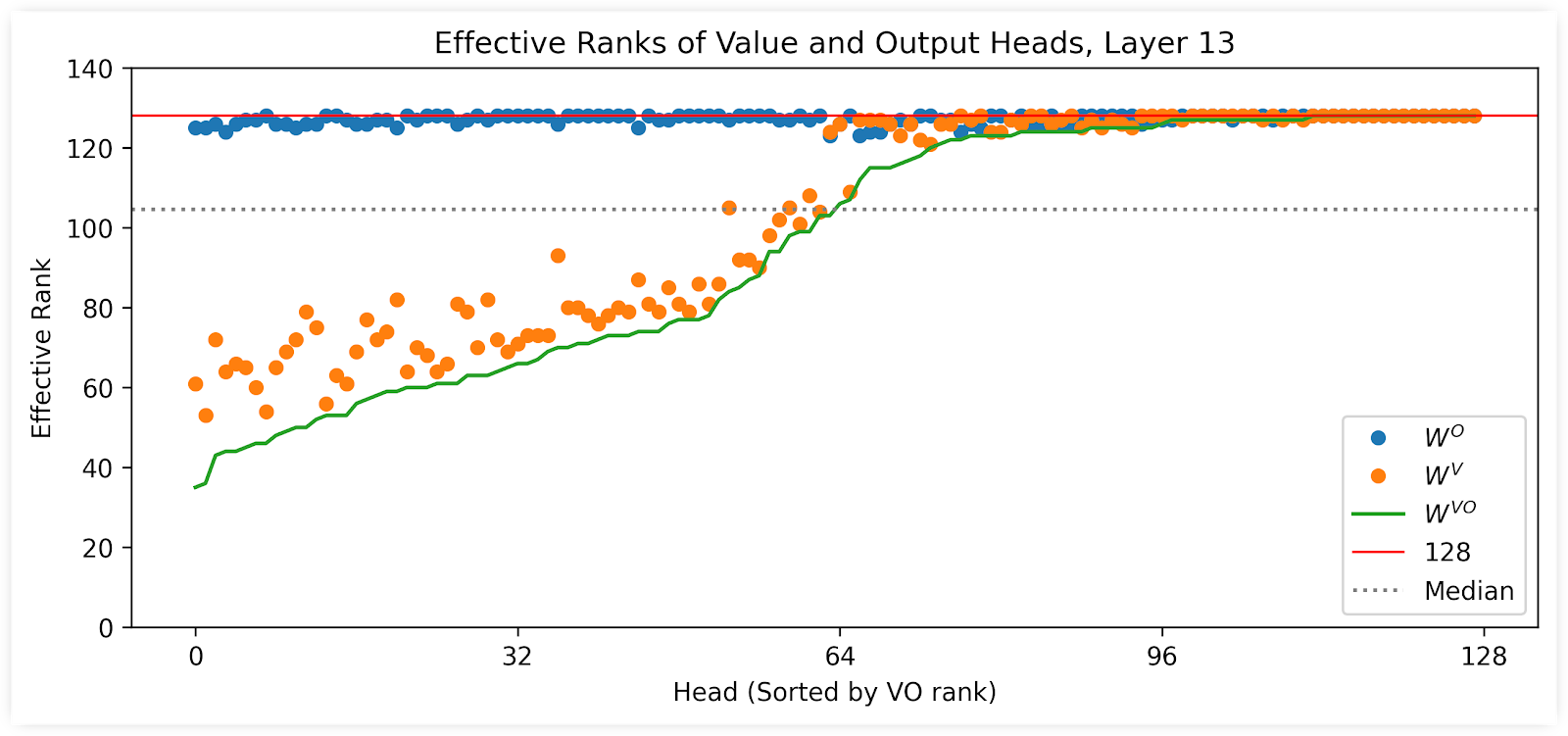
A number of interesting things to note here.
- Note how the green line–the effective rank of the fused matrix–is not only the minimum of the two matrices, but often even lower as well.
- The gap between the green line and the orange dots represents how much additional low-rank-ness was uncovered by fusing.
- Note how the Output heads have consistently high rank, and it’s the Value projections which are constraining the overall picture. This means that, in these cases, the Output has learned more distinct feature directions than the Value vectors can actually utilize.
For those first ~16 heads in the plot, it looks like we could comfortably take just the top 64 singular vectors from SVD and cut the size of those heads in half, and still have almost exactly the same behavior as the originals.
This analysis is pretty interesting to look at for the Query-Key heads as well, but I’ll save that for another post.
Also, the rank of individual heads isn’t what we’re currently interested in–we want to find common directions across all of the heads, so let’s get back to that perspective.
The Value-Output fusing needs to occur at a per-head level, but then we can stack the matrices again and compare them to the original $W^O$ per-layer.
Note: The fused version of the matrix is just for analysis. Once the analysis is done and we’ve found our subspaces, we’ll separate the heads again and decompose them back into separate Value and Output heads. By definition, the total error will be the same as what we see for the fused version.
I’ve previously dubbed this technique “Fuse and Rank Reduce” (FaRR)–we’ll see if that gains any traction.
The below plot shows the effective rank at 0.1% error of the fused $W^{VO}$ matrices versus just $W^O$.

The gains are quite impressive for those early layers! It’s also a little interesting to see how the rank dips again in the last handful of layers, the final layer in particular–something to explore.
But, the bulk of the model shows very little change. If you run the previous all-heads-in-a-layer plot on one of those middle layers, e.g., layer 25, both the value and output projections are close to full rank for all heads, and that’s clearly reflected here as well.
Implications
Overall, it seems clear that constraining the output heads to a single shared projection of size 3,072, or even 4,096, isn’t going to work well on the pre-trained DS-V3 model.
I think there’s still reason to suspect that a pre-trained model could do well with such a constraint though, beyond just the “intuitive” argument.
First, we can flip the problem around and ask–how much error would it incur to constrain the heads to a rank of 4,096 (which yields an 18% reduction in parameters and flops)?

Besides that one outlier (which seems interesting to investigate!) The error stays below 7%.
Second, I’ve had more “success” (only as evidenced by energy plots) when I first cluster the heads and then define multiple shared subspaces within those groups. That technique will be the subject of a coming post.
Conclusion
Here’s what I think we’ve found so far.
As far as making the existing pre-trained DeepSeek-V3 model more efficient with this approach:
- It’s unlikely to perform well with a shared output subspace in most layers.
- There are clear opportunities for compression in the early layers, and perhaps even some insights to gain relating to model training.
- In addition to a shared output subspace, it may be possible to reduce the size of many of the heads in the early layers, if we can do it in a way that doesn’t break GPU efficiency.
- Fusing the $W^V$ and $W^O$ matrices seems to significantly increase the opportunity for compression, where it exists.
For pre-training a new model:
- An error rate of 5-7% (<5% for Kimi-K2, see Appendix) for a compression rank of 4,096 may be evidence that the model will still learn well under this constraint.
Next Steps
- To explore the impact on pre-training,
- I started with training a small Vision Transformer (ViT) from scratch on the CIFAR-10 dataset, which seemed to work well.
- I moved on to training some tiny-scale Encoder models and benmarking on SST-2, you can see the code and preliminary results here.
- I also explored clustering the output heads of DS-V3 to see if the effective rank within the groups is low enough to consider creating a factorized version of the model, but nothing to share there yet.
Appendix
Code
You can find all of the code for the SVD analysis, along with a deeper dive into the overall technique, here.
Results on Kimi-K2
The more recent Kimi-K2 model from Moonshot AI uses the same architecture as DeepSeek-V3 but with:
- 64 heads instead of 128
- 384 experts vs. 256
- One dense layer instead of 3
The below plot shows the effective rank of the stacked $W^O$ matrices in every layer of Kimi-K2 at 1% and .1% error. Comparing this to the same analysis on DS-V3 earlier in this post, the effective rank is consistently lower.

As a result, the reconstruction error of the stacked $W^VO$ matrices at rank 4096 is also consistently lower.

Equations
Here are the updated equations for a single token vector $x \in \mathbb{R}^{d_\text{model}}$ passing through a Multihead Latent Attention (MLA) layer with the proposed Output latent space. I’m excluding the RoPE heads for now for brevity.
(Note that there is a summary table of the variables with example dimensions at the end).
1. Shared Latent Projections
First, the input token vector $x$ is projected down into two smaller, shared latent spaces: one for the Queries and one for the Keys and Values.
\[c_q = x W^{QA} \quad \in \mathbb{R}^{d_\text{latent_q}} \\ c_{kv} = x W^{KVA} \quad \in \mathbb{R}^{d_\text{latent_kv}}\]Where
\[W^{QA} \in \mathbb{R}^{d_\text{model} \times d_\text{latent_q}} \\ W^{KVA} \in \mathbb{R}^{d_\text{model} \times d_\text{latent_kv}}\]2. Per-Head Projections
Next, the latent vectors $c_q$ and $c_{kv}$ are used as input to the individual attention heads. For each head $i$ out of $h$ total heads:
\[q_i = c_q W^{QB}_i \\ k_i = c_{kv} W^{KB}_i \\ v_i = c_{kv} W^{VB}_i\]Where:
\[W^{QB}_i \in \mathbb{R}^{d_\text{latent_q} \times d_\text{query}} \\ W^{KB}_i \in \mathbb{R}^{d_\text{latent_kv} \times d_\text{key}} \\ W^{VB}_i \in \mathbb{R}^{d_\text{latent_kv} \times d_\text{value}}\]3. Scaled Dot-Product Attention
Attention scores are calculated for each head $i$ using the standard scaled dot-product attention mechanism. The output of this step for head $i$ is a scored value vector $z_i \in \mathbb{R}^{d_\text{value}}$:
\[z_i = \text{softmax}\left(\frac{q_i k_i^\top}{\sqrt{d_\text{key}}} \right) v_i\]4. Output Projections
The attended value vectors $z_i$ from all heads are concatenated and then projected into the output latent space using the projection matrix $W^{OA} \in \mathbb{R}^{h \cdot d_\text{value} \times d_\text{latent_o}}$:
\[c_o = \text{Concat}(z_1, z_2, \dots, z_h) W^{OA} \quad \in \mathbb{R}^{d_\text{latent_o}}\]This operation combines the per-head up projection and the summation across heads. It is equivalent to:
\[c_o = \sum_{i=1}^{h} \left(z_i W^{OA}_i \right)\]Where $W^{OA}i \in \mathbb{R}^{d{value} \times d_\text{latent_o}}$ is the per-head projection into output latent space.
Finally, the ouput latent is re-projected back into model space via a shared projection, giving the final output of the attention layer:
\[o = c_oW^{OB} \quad \in \mathbb{R}^{d_\text{model}}\]where $W^{OB} \in \mathbb{R}^{d_\text{latent_o} \times d_\text{model}}$ is the shared output projection into model space.
Summary of Variables
Example dimensions are taken from DeepSeek-V3 (except for the output latent dimension).
| Variable | Description | Example Dimensions |
|---|---|---|
| $x$ | Input token vector | $1 \times 7168$ |
| $d_\text{model}$ | Model (token vector) dimension | $7168$ |
| $d_\text{latent_q}$ | Query latent space dimension | $1536$ |
| $d_\text{latent_kv}$ | Key/Value latent space dimension | $512$ |
| $d_\text{latent_o}$ | Output latent space dimension | $1280$ |
| $d_\text{query}, d_\text{key}, d_\text{value}$ | Per-head dimensions | $128$ |
| $h$ | Number of heads | $128$ |
| $W^{QA}$ | Shared Query latent projection | $7168 \times 1536$ |
| $W^{KVA}$ | Shared Key/Value latent projection | $7168 \times 512$ |
| $W^{QB}_i$ | Per-head Query projection | $1536 \times 128$ |
| $W^{KB}_i$ | Per-head Key projection | $512 \times 128$ |
| $W^{VB}_i$ | Per-head Value projection | $512 \times 128$ |
| $W^{OA}_i$ | Per-head Output latent projection | $128 \times 1280$ |
| $W^{OB}$ | Shared Output projection | $1280 \times 7168$ |
Note: Kimi-K2 uses the same model, head, and latent sizes, but with only 64 heads instead of 128.