Product Quantizers for k-NN Tutorial Part 2
In part 1 of this tutorial, I described the most basic form of a product quantizer. In this post, I’ll be explaining the IndexIVFPQ index from the FAISS library, which uses a product quantizer as well as a couple additional techniques introduced in their 2011 paper.
Here is a brief summary of the two added features, followed by more detailed explanations.
Inverted File Index (IVF) The IVF is simply a technique for pre-filtering the dataset so that you don’t have to do an exhaustive search of all of the vectors. It’s pretty straightforward–you cluster the dataset ahead of time with k-means clustering to produce a large number (e.g., 100) of dataset partitions. Then, at query time, you compare your query vector to the partition centroids to find, e.g., the 10 closest clusters, and then you search against only the vectors in those partitions.
Encoding Residuals This is an enhancement to the basic product quantizer which incorporates information from the IVF step. For each database vector, instead of using the PQ to encode the original database vector we instead encode the vector’s offset from its partition centroid. I’ll explain why this works, and how it helps, in that section.
Inverted File Index
In Computer Science, and in Information Retrieval in particular, an “inverted index” refers to a text search index which maps every word in the vocabulary to all of its locations in all of the documents in the database. It’s a lot like the index you’d find in the back of a textbook, mapping words or concepts to page numbers, so it’s always bugged me that they call this data structure an inverted index (cause it seems like a normal index to me!).
Anyhow, in this context, the technique really just means partitioning the dataset using k-means clustering so that you can refine your search to only some of the partitions and ignore the rest.
As part of building the index, you use k-means clustering to cluster the dataset into a large number of partitions. Each vector in the dataset now belongs to one (and only one) of these clusters / partitions. And for each partition, you have a list of all the vectors that it contains (these are the “inverted file lists” referred to by the authors). You also have a matrix of all of the partition centroids, which will be used to figure out which partitions to search.
Dividing the dataset up this way isn’t perfect, because if a query vector falls on the outskirts of the closest cluster, then it’s nearest neighbors are likely sitting in multiple nearby clusters. The solution to this issue is simply to search multiple partitions. Searching multiple nearby partitions obviously takes more time, but gives us better accuracy.
At search time, you compare your query vector to all of the partition centroids to find the closest ones. Exactly how many is configurable. Once you’ve found the closest centroids, you select only the dataset vectors from those partitions, and do your k-NN search using the product quantizer.
A few notes on terminology:
- The verb “probe” is used in this context to refer to selecting partitions to search. So in the code you’ll see the index parameter “nprobe” meaning “number of partitions to probe”.
- The authors of FAISS like to use the term Voronoi cells (instead of “dataset partitions”, as I’ve been using). A Voronoi cell is just the region of space that belongs to a cluster. That is, it covers all the points in space where a vector would be closer to that cluster’s centroid than any other.
Encoding Residuals
This step is also relatively straightforward, but seems strange until you understand it. The idea is to incorporate some of the information from the IVF step into the product quantizer to improve its accuracy (so this concept definitely builds on top of the dataset partitioning technique).
First let’s define what a ‘residual’ vector is. And let’s tear out the product quantizer for now since it complicates things–we’ll add it back in later. That is, pretend we’re doing standard brute-force k-NN, but using the dataset partitioning technique to cut down on the number of vectors we search.
Let’s say you’ve clustered your dataset with k-means and now you have 100 clusters (or “dataset partitions”). For a given dataset vector, its residual is its offset from its partition centroid. That is, take the dataset vector and subtract from it the centroid vector of the cluster it belongs to. The centroid is just the mean of the cluster, so what happens when you subtract the mean from a collection points? They’re now all centered around 0. Here’s a simple two dimensional example.
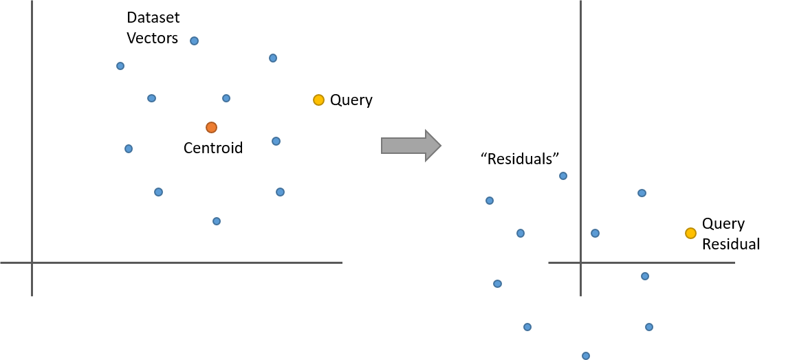
So here’s something interesting. Let’s say you replace all of the vectors in a partition with their residuals as in the above illustration. If you now have a query vector, and you want to find its nearest neighbors within this partition, you can calculate the query vector’s residual (it’s offset from the partition centroid), and then do your nearest neighbor search against the dataset vector residuals. And you’ll get the same result as using the original vectors!
I think you can see this intuitively in the illustration, but let’s also look at the equation. The L2 distance between two vectors ‘x’ and ‘y’, each of length ‘n’, is given by:
\[dist_{L2} ( {x}, {y} ) = \sqrt{\sum_{i}^{n}\left ( x_{i} - y_{i} \right )^{2}}\]What happens if we subtract a centroid vector ‘c’ from both ‘x’ and ‘y’?
\[dist_{L2} (x - c, y - c) = \sqrt{\sum_{i}^{n}\left ( \left ( x_{i} - c_{i} \right ) - \left ( y_{i} - c_{i} \right )\right )^{2}} = \sqrt{\sum_{i}^{n}\left ( x_{i} - y_{i} \right )^{2}}\]The centroid components just cancel out!
So note that this means that the distances calculated using the residuals are not only equivalent in relative terms (like the order of the distances), but we’re actually still calculating the correct L2 distance between the vectors!
You’ve probably already relied on this equivalence before, since mean normalization (subtracting the mean from your vectors) is a common pre-processing technique.
So that’s within a single partition, but what about comparing against vectors in different partitions? We’re still good, so long as we re-calculate the query vector residual for each partition.
Take a look at the following illustration with two partitions. After calculating the residuals, all of the points from both partitions are now centered around 0. But now we have two query vector residuals–one for comparing against the blue points (partition 1) and another for the green points (partition 2).
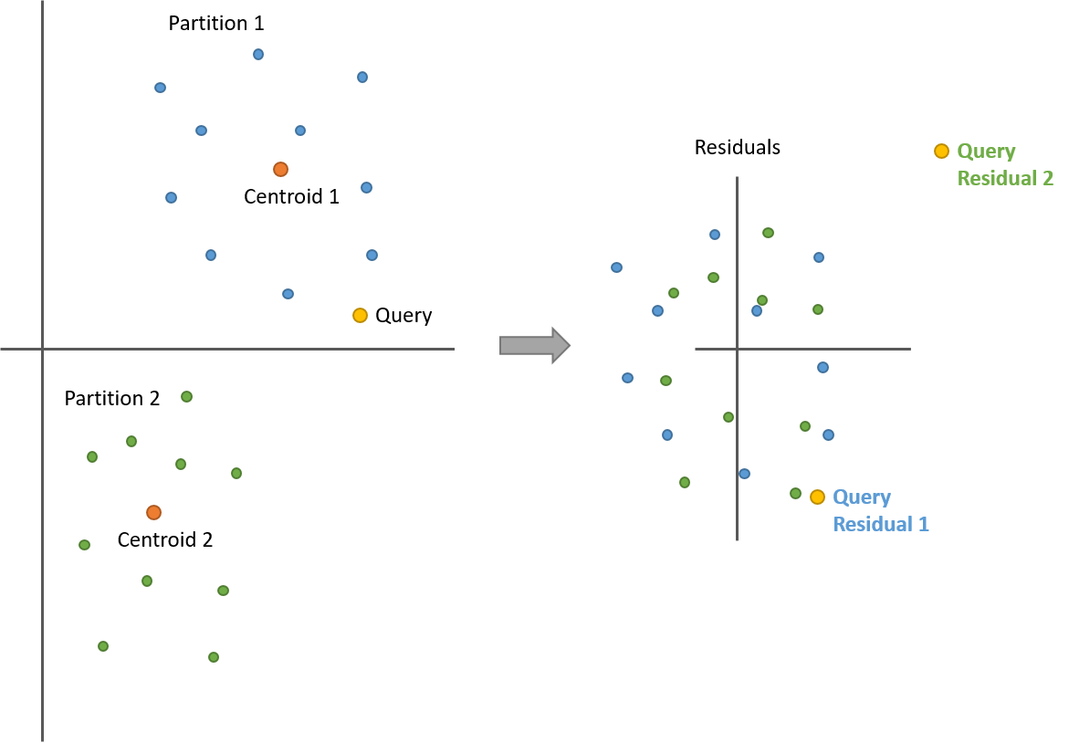
Note how the distances between the query and the points are still the same before and after!
So this is all very interesting, but so far useless. We haven’t changed our accuracy or reduced the compute burden at all. To see where we benefit from this, we have to bring the PQ back in to the picture.
Before training our product quantizer, we’re first going to calculate the residuals for all of the dataset vectors across all of the partitions. We’re still going to keep the residuals separated by partition (we’re not combining them), but now all of these residuals are all centered around 0, and relatively tightly grouped. And we’re actually going to toss the original dataset vectors, and just store the residuals from here on out.
Now we learn a product quantizer on all of these residual vectors instead of the original vectors. So what’s changed? Remember that the product quantizer works by dividing up the vectors into subvectors, and running k-means clustering on them to learn a set of prototypes (or a “code book”) to use to represent all of the vectors. What we’ve done by replacing the vectors with their residuals is that we’ve reduced the variety in the dataset (In the paper, this is described by saying that the residual vectors “have less energy” than the originals.). Where before the clusters were all in different regions of space, now all of the clusters are centered around 0 and overlapping one another. By reducing the variety in the dataset, it takes fewer prototypes (or “codes”) to represent the vectors effectively! Or, from another perspective, our limited number of codes in the PQ are now going to be more accurate because the vectors they have to describe are less distinct than they were. We’re getting more bang for our buck!
There is a cost to this, though. Remember that the magic of Product Quantizers is that you only have to calculate a relatively small table of partial distances between the query vector chunks and the codes in the codebooks–the rest is look-ups and summations.
But now with the residuals, the query vector is different for each partition–in each partition, the residual for the query has to be re-calculated against that partition’s centroid. So we have to calculate a separate distance table for each partition we probe!
Apparently the trade-off is worth it, though, because the IndexIVFPQ works pretty well in practice.
And that’s really it. The database vectors have all been replaced by their residuals, but from the perspective of the Product Quantizer nothing’s different.
Note that the partitions don’t factor in to the codebook training. We still learn a codebook for each subvector using dataset vectors across all partitions. You could train separate PQs for each partition, but the authors decided against this because the number of partitions tends to be high, so the memory cost of storing all those codebooks is a problem. Instead, a single PQ is still learned from all of the database vectors from all partitions.