Gaussian Mixture Models Tutorial and MATLAB Code
You can think of building a Gaussian Mixture Model as a type of clustering algorithm. Using an iterative technique called Expectation Maximization, the process and result is very similar to k-means clustering. The difference is that the clusters are assumed to each have an independent Gaussian distribution, each with their own mean and covariance matrix.
Comparison To K-Means Clustering
When performing k-means clustering, you assign points to clusters using the straight Euclidean distance. The Euclidean distance is a poor metric, however, when the cluster contains significant covariance. In the below example, we have a group of points exhibiting some correlation. The red and green x’s are equidistant from the cluster mean using the Euclidean distance, but we can see intuitively that the red X doesn’t match the statistics of this cluster near as well as the green X.
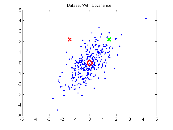
If you were to take these points and normalize them to remove the covariance (using a process called whitening), the green X becomes much closer to the mean than the red X.

The Gaussian Mixture Models approach will take cluster covariance into account when forming the clusters.
Another important difference with k-means is that standard k-means performs a hard assignment of data points to clusters–each point is assigned to the closest cluster. With Gaussian Mixture Models, what we will end up is a collection of independent Gaussian distributions, and so for each data point, we will have a probability that it belongs to each of these distributions / clusters.
Expectation Maximization
For GMMs, we will find the clusters using a technique called “Expectation Maximization”. This is an iterative technique that feels a lot like the iterative approach used in k-means clustering.
In the “Expectation” step, we will calculate the probability that each data point belongs to each cluster (using our current estimated mean vectors and covariance matrices). This seems analogous to the cluster assignment step in k-means.
In the “Maximization” step, we’ll re-calculate the cluster means and covariances based on the probabilities calculated in the expectation step. This seems analogous to the cluster movement step in k-means.
Initialization
To kickstart the EM algorithm, we’ll randomly select data points to use as the initial means, and we’ll set the covariance matrix for each cluster to be equal to the covariance of the full training set. Also, we’ll give each cluster equal “prior probability”. A cluster’s “prior probability” is just the fraction of the dataset that belongs to each cluster. We’ll start by assuming the dataset is equally divided between the clusters.
Expectation
In the “Expectation” step, we calculate the probability that each data point belongs to each cluster.
We’ll need the equation for the probability density function of a multivariate Gaussian. A multivariate Gaussian (“multivariate” just means multiple input variables) is more complex because there is the possibility for the different variables to have different variances, and even for there to be correlation between the variables. These properties are captured by the covariance matrix.
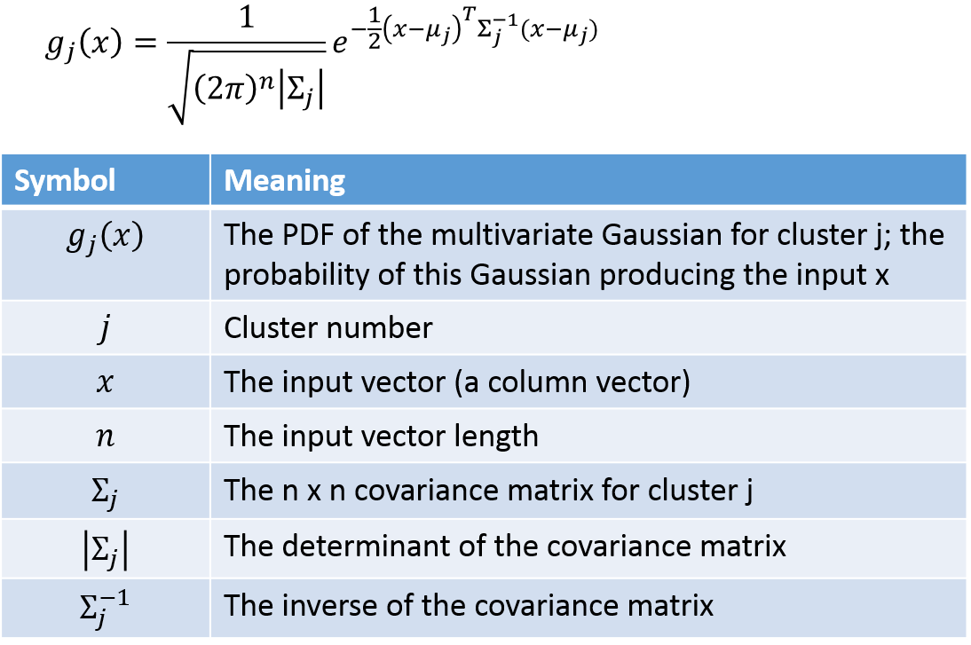
The probability that example point i belongs to cluster j can be calculated using the following:
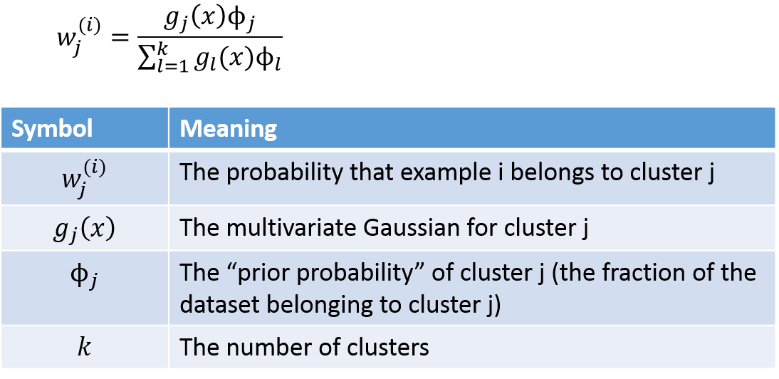
We’ll apply this equation to every example and every cluster, giving us a matrix with one row per example and one column per cluster.
Maximization
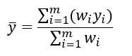
You can gain some useful intuition about the maximization equations if you’re familiar with the equation for taking a weighted average. To find the average value of a set of m values, where you have a weight _w _defined for each of the values, you can use the following equation:
With this in mind, the update rules for the maximization step are below. I’ve copied these from the lecture notes on GMMs for Stanford’s CS229 course on machine learning (those lecture notes are a great reference, by the way).
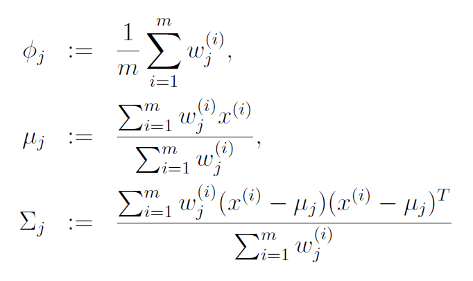
The equation for mean (mu) of cluster j is just the average of all data points in the training set, with each example weighted by its probability of belonging to cluster j.
Similary, the equation for the covariance matrix is the same as the equation you would use to estimate the covariance of a dataset, except that the contribution of each example is again weighted by the probability that it belongs to cluster j.
The prior probability of cluster j, denoted as phi, is calculated as the average probability that a data point belongs to cluster j.
MATLAB Example Code
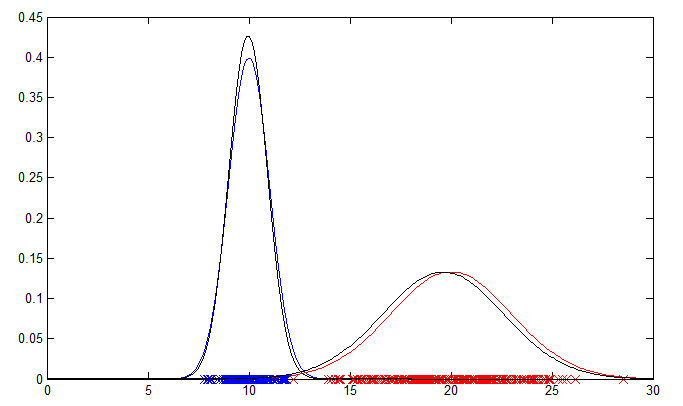
I’ve implemented Expectation Maximization for both a 1D and a 2D example. Run ‘GMMExample_1D.m’ and ‘GMMExample_2D.m’, respectively. The 1D example is easier to follow, but the 2D example can be extended to n-dimensional data.
If you are simply interested in using GMMs and don’t care how they’re implemented, you might consider using the vlfeat implementation, which includes a nice tutorial here. Or if you are using Octave, there may be an open-source version of Matlab’s ‘fitgmdist’ function from their Statistics Toolbox.
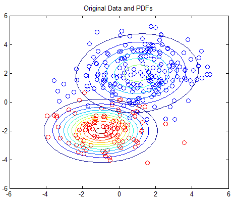
The 1D example will output a plot showing the original data points and their PDFs in blue and red. The PDFs estimated by the EM algorithm are plotted in black for comparison.
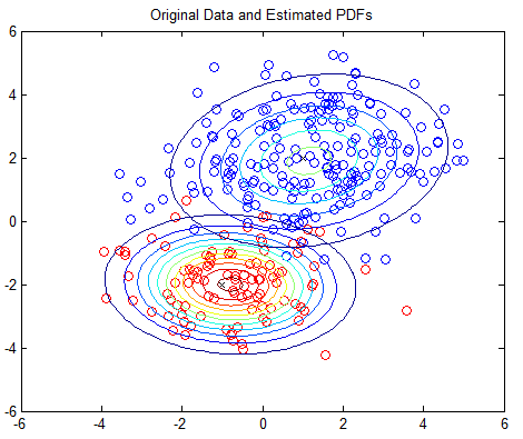
The 2D example is based on Matlab’s own GMM tutorial here, but without any dependency on the Statistics Toolbox. The 2D example plots the PDFs using contour plots; you should see one plot of the original PDFs and another showing the estimated PDFs.