Gradient Descent Derivation

Andrew Ng’s course on Machine Learning at Coursera provides an excellent explanation of gradient descent for linear regression. To really get a strong grasp on it, I decided to work through some of the derivations and some simple examples here.

This material assumes some familiarity with linear regression, and is primarily intended to provide additional insight into the gradient descent technique, not linear regression in general.

I am making use of the same notation as the Coursera course, so it will be most helpful for students of that course.

For linear regression, we have a linear hypothesis function, $h(x) = \theta_0 + \theta_1 x$. We want to find the values of $\theta_0$ and $\theta_1$ which provide the best fit of our hypothesis to a training set. The training set examples are labeled $x, y$, where $x$ is the input value and $y$ is the output. The ith training example is labeled as $x^{(i)}, y^{(i)}$. Do not confuse this as an exponent! It just means that this is the ith training example.

MSE Cost Function

The cost function $J$ for a particular choice of parameters $\theta$ is the mean squared error (MSE):

Where the variables used are:

The MSE measures the average amount that the model’s predictions vary from the correct values, so you can think of it as a measure of the model’s performance on the training set. The cost is higher when the model is performing poorly on the training set. The objective of the learning algorithm, then, is to find the parameters $\theta$ which give the minimum possible cost $J$.

This minimization objective is expressed using the following notation, which simply states that we want to find the $\theta$ which minimizes the cost $J(\theta)$.

Gradient Descent Minimization - Single Variable Example

We’re going to be using gradient descent to find $\theta$ that minimizes the cost. But let’s forget the MSE cost function for a moment and look at gradient descent as a minimization technique in general.

Let’s take the much simpler function $J(\theta) = {\theta}^2$, and let’s say we want to find the value of $\theta$ which minimizes $J(\theta)$.

Gradient descent starts with a random value of $\theta$, typically $\theta = 0$, but since $\theta = 0$ is already the minimum of our function ${\theta}^2$, let’s start with $\theta = 3$.

Gradient descent is an iterative algorithm which we will run many times. On each iteration, we apply the following “update rule” (the := symbol means replace theta with the value computed on the right):

Alpha is a parameter called the learning rate which we’ll come back to, but for now we’re going to set it to 0.1. The derivative of $J(\theta)$ is simply $2\theta$.

Below is a plot of our function, $J(\theta)$, and the value of $\theta$ over ten iterations of gradient descent.

Below is a table showing the value of theta prior to each iteration, and the update amounts.

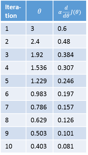
Cost Function Derivative

Why does gradient descent use the derivative of the cost function? Finding the slope of the cost function at our current $\theta$ value tells us two things.

The first is the direction to move theta in. When you look at the plot of a function, a positive slope means the function goes upward as you move right, so we want to move left in order to find the minimum. Similarly, a negative slope means the function goes downard towards the right, so we want to move right to find the minimum.

The second is how big of a step to take. If the slope is large we want to take a large step because we’re far from the minimum. If the slope is small we want to take a smaller step. Note in the example above how gradient descent takes increasingly smaller steps towards the minimum with each iteration.

The Learning Rate - Alpha

The learning rate gives the engineer some additional control over how large of steps we make.

Selecting the right learning rate is critical. If the learning rate is too large, you can overstep the minimum and even diverge. For example, think through what would happen in the above example if we used a learning rate of 2. Each iteration would take us farther away from the minimum!

The only concern with using too small of a learning rate is that you will need to run more iterations of gradient descent, increasing your training time.

Convergence / Stopping Gradient Descent

Note in the above example that gradient descent will never actually converge on the minimum, $\theta = 0$. Methods for deciding when to stop gradient descent are beyond my level of expertise, but I can tell you that when gradient descent is used in the assignments in the Coursera course, gradient descent is run for a large, fixed number of iterations (for example, 100 iterations), with no test for convergence.

Gradient Descent - Multiple Variables Example

The MSE cost function includes multiple variables, so let’s look at one more simple minimization example before going back to the cost function.

Let’s take the function:

When there are multiple variables in the minimization objective, gradient descent defines a separate update rule for each variable. The update rule for $\theta_1$ uses the partial derivative of $J$ with respect to $\theta_1$. A partial derivative just means that we hold all of the other variables constant–to take the partial derivative with respect to $\theta_1$, we just treat $\theta_2$ as a constant. The update rules are in the table below, as well as the math for calculating the partial derivatives. Make sure you work through those; I wrote out the derivation to make it easy to follow.

Note that when implementing the update rule in software, $\theta_1$ and $\theta_2$ should not be updated until after you have computed the new values for both of them. Specifically, you don’t want to use the new value of $\theta_1$ to calculate the new value of $\theta_2$.

Gradient Descent of MSE

Now that we know how to perform gradient descent on an equation with multiple variables, we can return to looking at gradient descent on our MSE cost function.

The MSE cost function is labeled as equation [1.0] below. Taking the derivative of this equation is a little more tricky. The key thing to remember is that x and y are not variables for the sake of the derivative. Rather, they represent a large set of constants (your training set). So when taking the derivative of the cost function, we’ll treat x and y like we would any other constant.

Once again, our hypothesis function for linear regression is the following:

I’ve written out the derivation below, and I explain each step in detail further down.

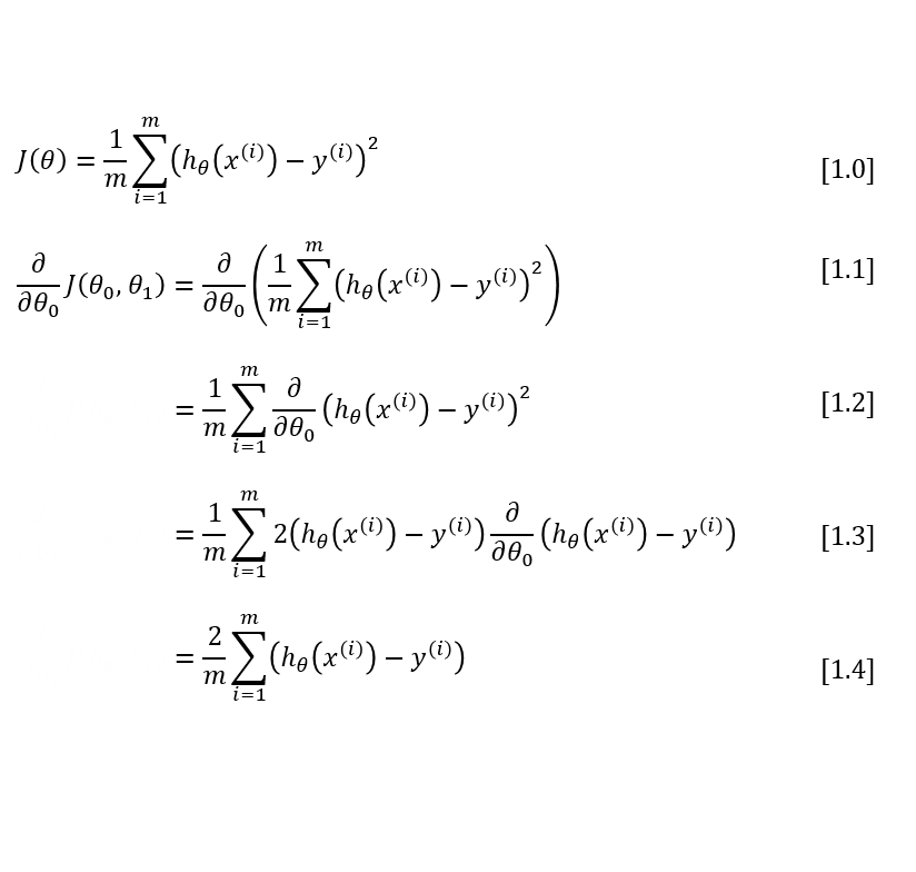
To move from equation [1.1] to [1.2], we need to apply two basic derivative rules:

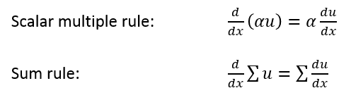
Moving from [1.2] to [1.3], we apply both the power rule and the chain rule:

Finally, to go from [1.3] to [1.4], we must evaluate the partial derivative as follows. Recall again that when taking this partial derivative all letters except $\theta_0$ are treated as constants ( $\theta_1$, $x$, and $y$).

Equation [1.4] gives us the partial derivative of the MSE cost function with respect to one of the variables, $\theta_0$. Now we must also take the partial derivative of the MSE function with respect to $\theta_1$. The only difference is in the final step, where we take the partial derivative of the error:

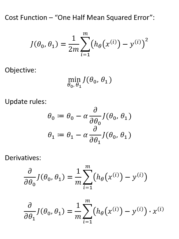
One Half Mean Squared Error

In Andrew Ng’s Machine Learning course, there is one small modification to this derivation. We multiply our MSE cost function by 1/2 so that when we take the derivative, the 2s cancel out. Multiplying the cost function by a scalar does not affect the location of its minimum, so we can get away with this.

Alternatively, you could think of this as folding the 2 into the learning rate. It makes sense to leave the 1/m term, though, because we want the same learning rate (alpha) to work for different training set sizes (m).

Final Update Rules

Altogether, we have the following definition for gradient descent over our cost function.

Training Set Statistics

Note that each update of the theta variables is averaged over the training set. Every training example suggests its own modification to the theta values, and then we take the average of these suggestions to make our actual update.

This means that the statistics of your training set are being taken into account during the learning process. An outlier training example (or even a mislabeled / corrupted example) is going to have less influence over the final weights because it is one voice versus many.