Deep Learning Tutorial - Softmax Regression

Softmax regression is a generalized form of logistic regression which can be used in multi-class classification problems where the classes are mutually exclusive. The hand-written digit dataset used in this tutorial is a perfect example. A softmax regression classifier trained on the hand written digits will output a separate probability for each of the ten digits, and the probabilities will all add up to 1.

Softmax regression consists of ten linear classifiers of the form:

The output of this equation is a vector, with one value for each hand-written digit. The first component is the probability that an input image of a digit, x, is the number “1” (belongs to class y = 1).

The tutorial notes don’t show this classifier is derived, and the relationship between this equation and the original binary logistic regression classifier is certainly not obvious.

One bit of intuition you can derive about it, though, is the normalization. By dividing each component by the sum of all the components, we ensure that the sum of all the elements in the vector will always equal 1. This makes sense given that the classes are all mutually exclusive.

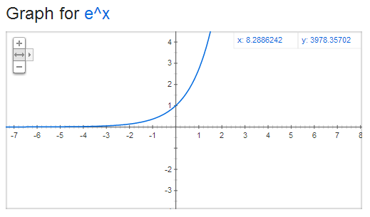
Below is the plot of e^x. There’s not much intuition to be derived from this plot, other than that the output of e^x is always positive.

Over-Parameterization

The tutorial makes the point that you could fix the vector of parameters for one of the 10 classifiers (say, theta_1) to a vector of all zeros, and the classifier would still be able to function by learning the parameters for the other 9 classifiers.

How is this possible? If you were to set theta_1 to all zeros, then the first component of the un-normalized output vector would always be equal to 1, no matter what the input is.

However, the normalization allows this component to take on different values depending on the un-normalized outputs of the other 9 classifiers.

Logistic Regression as a Specific Case of Softmax Regression

While the notes don’t provide a derivation of Softmax Regression, they do show how you can arrive at logistic regression by looking at the special case of Softmax Regression with two classes.

Cost Function

Below is the cost function (with weight decay) for Softmax Regression from the tutorial.

The indicator function denoted by 1{y^(i) = j} means that only the output of the classifier corresponding to the correct class label is included in the cost. That is, when computing the cost for an example of the digit “4”, only the output of classifier 4 contributes to the cost.

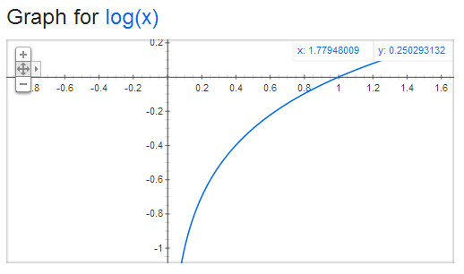
Below is a plot of log(x). Note that the input will only range from 0 to 1. The costs in this range are all negative, so note the negative sign at the beginning of our cost function to account for this.

The output of log(x) ranges from negative infinity to 0. If the classifier outputs 1 for the training example, then the cost is zero. The cost increases exponentially as the classifier’s output decreases towards 0. Sounds like good behavior for our cost function!

Gradients

Below is the gradient function from the tutorial.

Note that this function computes the gradients for a single class j. The expression inside the parentheses evaluates to a single value between 0 and 1. This is multiplied by the vector x^(i) to get the weight updates for a single training example i and a single class j.

Let’s say that you evaluate the inner expression for every class and every training example, such that you have a matrix M which is [numClasses x numExamples].

We want a gradient matrix ‘grad’ which is [numClasses x inputSize]. We also have our data matrix ‘data’ which is [inputSize x numExamples].

To compute the ‘grad’ matrix for all examples and all classes simultaneously, we compute

grad = M * data’

You can confirm that the dimensions match up:

grad [numClasses x inputSize] = M [numClasses x numExamples] * data’ [numExamples x inputSize]

To calculate the final gradient matrix, you also need to take the average of these gradients by dividing them by the number of training examples. Finally, you need to add in the regularization term of the gradient.

Softmax Regression Exercise

This exercise is considerably easier than the sparse auto-encoder.

Since the first step of calculating the cost is to evaluate the model over the training set, I recommend starting by completing the ‘softmaxPredict.m’ function. I modified my version of softmaxPredict to return both the class labels and the matrix of confidences so that I could call it from my ‘softmaxCost.m’ function.

Note for Octave Users

Octave does not support ‘mex’ files, so you will need to add the line “options.useMex = false;” before calling minFunc in softmaxTrain.m.

Fortunately, memory was not an issue for this exercise–I was able to run the full 100 training iterations.