Interpreting LSI Document Similarity

In this post I’m sharing a technique I’ve found for showing which words in a piece of text contribute most to its similarity with another piece of text when using Latent Semantic Indexing (LSI) to represent the two documents. This has proven valuable to me in debugging bad search results from “concept search” using LSI. You’ll find the equations for the technique as well as example Python code.

My Fun NLP Project

I’ve been having a lot of fun playing with Latent Semantic Indexing (LSI) on a personal project. I’m working on making my personal journals, as well as some books I’ve read, searchable using LSI. That is, I can take one of my journal entries, and search for other journal entries (or even paragraphs from one of the books) that are conceptually similar.

I’m basing the project on the awesome “topic modeling” package gensim in Python. I’m sharing the fundamental code for this project (just not my journals :-P) on GitHub in a project I’ve called simsearch.

It also contains a working example based on the public domain work Matthew Henry’s Commentary on the Bible (which comes from the early 1700s!). I’ll show you some of that example a little farther down.

So far, though, the quality of the search results with my journals has been pretty hit-or-miss. For the really bad results, I’m left wondering, what went wrong?! Why does LSI think these two pieces of text are related? How can I interpret this match?

Impact of Each Word on Similarity

Turns out it’s possible to look at the impact of individual words on the total LSI similarity, allowing you to interpret the results some.

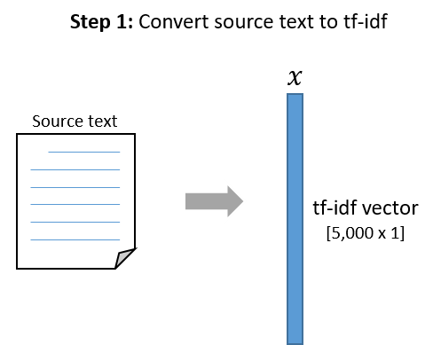
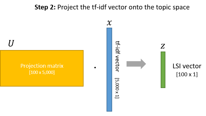
First, a little refresher on how LSI works. The first step in comparing the two pieces of text is to produce tf-idf vectors for them, which contain one element per word in the vocabulary. These tf-idf vectors are then projected down to, e.g., 100 topics with LSI. Finally, the two LSI vectors are compared using Cosine Similarity, which produces a value between 0.0 and 1.0.

Given that the tf-idf vectors contain a separate component for each word, it seemed reasonable to me to ask, “How much does each word contribute, positively or negatively, to the final similarity value?”

At first, I made some reckless attempts at modifying the code to give me what I wanted, but it became clear that the math wasn’t right–stuff wasn’t adding up right. So I had to bite the bullet and do some actual math :).

Originally I was hoping to calculate, for example, how the word ‘sabbath’ contributes to the total similarity, independent of which document it comes from. Turns out you can’t do exactly this, but you can do something close that I’m content with.

Instead of asking how the word ‘sabbath’ in both documents contributes to the total similarity, we can instead ask, how does the word ‘sabbath’ in document 1 contribute to its similarity with document 2?

I’ve shared the equations for this technique down in the next section. But first let’s look at the working result!

Working Example

In my simsearch project, I’ve included an example with Matthew Henry’s Commentary on the Bible. I take a section of the commentary on Genesis 2 which talks about the seventh day of creation, when God rested, and use this to search against the rest of the commentary. The top result is a great match–it’s commentary on Exodus 20, where God gives Moses the fourth commandment to remember the Sabbath, a day of rest. Definitely conceptually similar.

Using the technique I worked out, you can see how each word contributes to the total similarity value of 0.954 between these two pieces of text.

Here are the top 10 words in “document 1” (the commentary on Genesis) that contribute most to the similarity. If you add up all the terms, they sum to 0.954.

Total similarity: 0.954
Breakdown by word:
     sabbath    0.354
         day    0.315
      honour    0.032
        work    0.027
        rest    0.027
        holy    0.024
        week    0.015
     blessed    0.014
     seventh    0.013
        days    0.012
         ...

You can do the same for “document 2” (the commentary on the Ten Commandments). Again, if you sum all terms you get the total similarity of 0.954.

Total similarity: 0.954
Breakdown by word:
     sabbath    0.423
         day    0.250
        work    0.034
     seventh    0.032
        rest    0.017
        days    0.016
     blessed    0.016
        holy    0.010
    blessing    0.009
  sanctified    0.009
         ...

Note how the results are a little different taken from the perspective of document 1 vs. document 2. This is the compromise I mentioned earlier–you have to look at the two documents separately.

Equation for the Technique

First, let’s define our variables.

• \( x^{(1)} \) and \( x^{(2)} \) are the tf-idf vectors representing the two documents.
• \( z^{(1)} \) and \( z^{(2)} \) are the corresponding LSI vectors for these two documents.

To cut down on the number of variables, let’s assume that we have a vocabulary of 5,000 words (so our tf-idf vectors are 5,000 components long), and that we are using LSI with 100 topics (so our LSI vectors are 100 components long).

To calculate how much word \( j \) from document 1 contributes to the total similarity, we can use the following equation.

• \( U \) is the LSI project matrix which is [100 x 5,000].
• \( U_{*j} \) is the column for the word \( j \). This is [100 x 1]
• \( x_{j}^{(1)} \) is the tf-idf value in document 1 for word \( j \).
• \( z^{(2)} \) is the [100 x 1] LSI vector for document 2.
• \( \left| z^{(1)} \right| \) and \( \left| z^{(2)} \right| \) are the magnitudes of the two LSI vectors (recall that the Cosine Similarity involves normalizing the LSI vectors–dividing them by their magnitudes).

Derivation

To convert the tf-idf vector into an LSI vector, we just take the product of the [100 x 5,000] LSI projection matrix \( U \) and the [5,000 x 1] tfidf vector \( x \):

We want to look at the individual contribution of each word to our final similarity, so let’s expand the dot-product into the element-wise equation:

To calculate the similarity between our two documents, we compare their LSI vectors using the cosine similarity.

The cosine similarity between the vectors is found by normalizing them and taking their dot-product:

Let’s expand that dot product to see the element-wise operations:

This equation would allow us to see the similarity contribution for each of the 100 topics. However, what we really want is the similarity contribution from each word.

Time to make things a little nasty. Let’s substitute in our equation for \( z_{i} \) to put this equation in terms of the original tf-idf vectors.

What I originally wanted to do here was to see, for example, how the word ‘sabbath’ contributes to the total similarity, independent of which document it comes from. In order to do that, I would need to take the above equation and find a way to express it as a sum over \( j \). That way I could separate it into 5,000 terms, each term representing the similarity contribution from the corresponding word.

Problem is, I don’t think that’s possible. You would need to consolidate those two sums over \( j \). But “product of sums” is not the same as the “sum of products”.

There is an alternate solution, though, that seems perfectly acceptable to me. Instead of asking how the word ‘sabbath’ in both documents contributes to the total similarity, we can instead ask, how does the word ‘sabbath’ in document 1 contribute to its similarity with document 2?

We’re going to take a step backwards, and remove \( x^{(2)} \) from the equation.

By the distributive property, we can then move the \( z_{i}^{(2)} \) term into the sum:

Finally, by the commutative property of addition, we’re allowed to switch the order of those two sums:

We did it! We’ve managed to express the similarity between documents 1 and 2 as a sum of 5,000 terms. Now we can sort these terms to see which words in document 1 are contributing most to the total similarity.

If you want to look at just the contribution from a specific word \( j \) from document 1:

Or, in vector form:

Sample Code

You can find all of the Python code for the example I’ve discussed in my simsearch project on GitHub. Follow the instructions in the README to get it going. Note that there are a few dependencies you may have to grab if you don’t already have them, such as gensim and nltk.