Product Quantizers for k-NN Tutorial Part 1

• Exhaustive Search with Approximate Distances
• Explanation by Example
• Dataset Compression
• Nearest Neighbor Search
• Compression Terminology
• Pre-filtering

A product quantizer is a type of “vector quantizer” (I’ll explain what that means later on!) which can be used to accelerate approximate nearest neighbor search. They’re of particular interest because they are a key element of the popular Facebook AI Similarity Search (FAISS) library released in March 2017. In part 1 of this tutorial, I’ll be providing an explanation of a product quantizer in its most basic form, as used for implementing approximate nearest neighbors search (ANN). Then in part 2 I explain the “IndexIVFPQ” index from FAISS, which adds a couple more features on top of the basic product quantizer.

Exhaustive Search with Approximate Distances

Unlike tree-based indexes used for ANN, a k-NN search with a product quantizer alone still performs an “exhaustive search”, meaning that a product quantizer still requires comparing the query vector to every vector in the database. The key is that it approximates and greatly simplifies the distance calculations.

(Note that the IndexIVFPQ index in FAISS does perform pre-filtering of the dataset before using the product quantizer–I cover this in part 2).

Explanation by Example

The authors of the product quantizer approach have a background in signal processing and compression techniques, so their language and terminology probably feels foreign if your focus is machine learning. Fortunately, if you’re familiar with k-means clustering (and we dispense with all of the compression nomenclature!) you can understand the basics of product quantizers easily with an example. Afterwards, we’ll come back and look at the compression terminology.

Dataset Compression

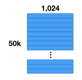
Let’s say you have a collection of 50,000 images, and you’ve already performed some feature extraction with a convolutional neural network, and now you have a dataset of 50,000 feature vectors with 1,024 components each.

The first thing we’re going to do is compress our dataset. The number of vectors will stay the same, but we’ll reduce the amount of storage required for each vector. Note that what we’re going to do is not the same as “dimensionality reduction”! This is because the values in the compressed vectors are actually symbolic rather than numeric, so we can’t compare the compressed vectors to one another directly.

Two important benefits to compressing the dataset are that (1) memory access times are generally the limiting factor on processing speed, and (2) sheer memory capacity can be a problem for big datasets.

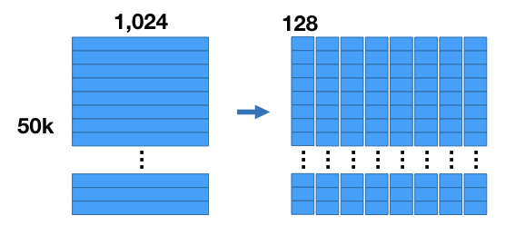
Here’s how the compression works. For our example we’re going to chop up the vectors into 8 sub-vectors, each of length 128 (8 sub vectors x 128 components = 1,024 components). This divides our dataset into 8 matrices that are [50K x 128] each.

We’re going to run k-means clustering separately on each of these 8 matrices with k = 256. Now for each of the 8 subsections of the vector we have a set of 256 centroids–we have 8 groups of 256 centroids each.

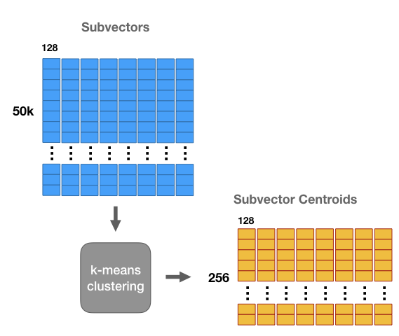
These centroids are like “prototypes”. They represent the most commonly occurring patterns in the dataset sub-vectors.

We’re going to use these centroids to compress our 1 million vector dataset. Effectively, we’re going to replace each subregion of a vector with the closest matching centroid, giving us a vector that’s different from the original, but hopefully still close.

Doing this allows us to store the vectors much more efficiently—instead of storing the original floating point values, we’re just going to store cluster ids. For each subvector, we find the closest centroid, and store the id of that centroid.

Each vector is going to be replaced by a sequence of 8 centroid ids. I think you can guess how we pick the centroid ids–you take each subvector, find the closest centroid, and replace it with that centroid’s id.

Note that we learn a different set of centroids for each subsection. And when we replace a subvector with the id of the closest centroid, we are only comparing against the 256 centroids for that subsection of the vector.

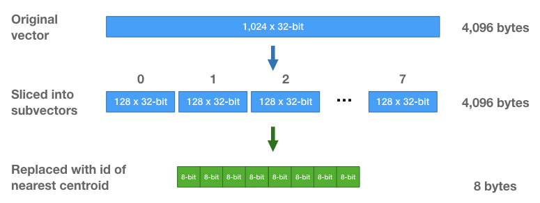
Because there are only 256 centroids, we only need 8-bits to store a centroid id. Each vector, which initially was a vector of 1,024 32-bit floats (4,096 bytes) is now a sequence of eight 8-bit integers (8 bytes total per vector!).

Nearest Neighbor Search

Great. We’ve compressed the vectors, but now you can’t calculate L2 distance directly on the compressed vectors–the distance between centroid ids is arbitrary and meaningless! (This is what differentiates compression from dimensionality reduction).

Here’s how we perform a nearest neighbor search. It’s still going to be an exhaustive search (we’re still going to calculate a distance against all of the vectors and then sort the distances) but we’re going to be able to calculate the distances much more efficiently using just table look-ups and some addition.

Let’s say we have a query vector and we want to find its nearest neighbors.

One way to do this (that isn’t so smart) would be to decompress the dataset vectors, and then calculate the L2 distances. That is, reconstruct the vectors by concatenating the different centroids. We’re effectively going to do this, but in a much more computationally efficient way than actually decompressing the vectors.

First, we’re going to calculate the squared L2 distance between each subsection of our vector and each of the 256 centroids for that subsection.

This means building a table of subvector distances with 256 rows (one for each centroid) and 8 columns (one foreach subsection). How much effort is it to build this table? If you think about it, this requires the same number of math operations as computing L2 distances between our query vector and 256 dataset vectors.

Once we have this table, we can start calculating approximate distance values for each of the 50K database vectors.

Remember that each database vector is now just a sequence of 8 centroid ids. To calculate the approximate distance between a given database vector and the query vector, we just use those centroid id’s to lookup the partial distances in the table, and sum those up!

Does it really work to just sum up those partial values? Yes! Remember that we’re just working with squared L2 distances, meaning no square root operation. Squared L2 is calculated by summing up all of squared differences between each component, so it doesn’t matter what order you perform those additions in.

So this table approach gives us the same result as calculating distances against the decompressed vectors, but with much lower compute cost.

The final step is the same as an ordinary nearest neighbor search—we sort the distances to find the smallest distances; these are the nearest neighbors. And that’s it!

Compression Terminology

Now that you understand how PQs work, it’s easy to go back and learn the terminology.

A quantizer, in the broadest sense, is something that reduces the number of possible values that a variable has. A good example would be building a lookup table to reduce the number of colors in an image. Find the most common 256 colors, and put them in a table mapping a 24-bit RGB color value down to an 8-bit integer.

When we took the first 128 values of our database vectors (the first of the 8 subsections) and clustered them to learn 256 centroids, these 256 centroids form what’s refered to as a “codebook”. Each centroid (a floating point vector with 128 components) is called a “code”.

Since these centroids are what’s used to represent the database vectors, the codes are also referred to as “reproduction values” or “reconstruction values”. You can reconstruct a database vector from its sequence of centroid if ids by concatenating the corresponding codes (centroids).

Since we ran k-means separately on each of the 8 subsections, we actually created eight separate code books.

With these 8 codebooks, though, we can combine the codes to create 256^8 possible vectors! So, in effect, we’ve created one very large codebook with 256^8 codes. Learning and storing a single codebook of that size directly is impossible, so that’s the magic of the product quantizer.

Pre-filtering

In part 2 of this tutorial, we’ll cover the IndexIVFPQ from FAISS, which uses a product quantizer but also partitions the dataset so that you only have to search through portions of it for each query. Though FAISS was just released in 2017, the product quantizer approach and the techniques used in the IndexIVFPQ were first introduced in their popular 2011 paper.