QLoRA and 4-bit Quantization

An in-depth tutorial on the algorithm and paper, including a pseudo-implementation in Python.

by Chris McCormick

S1. Introduction

QLoRA is really about a technique called “4-bit quantization”. It’s not a different version of “LoRA”, so the title can be confusing. We’ll see why LoRA is relevant, but let’s start with the more important part–representing weights with 4-bit values.

Getting LLM weights all the way down to 4-bits sounds pretty crazy, right? In Machine Learning, we’ve gone from using 32-bit floats, down to 16-bit floats, and now we’re all the way down to 4-bits per value?! 😲

Well… no. Sorry. When you apply 4-bit quantization to a 16-bit model, you don’t actually get a “4-bit model”–it’s still 16-bit!

Instead, this is simply a compression technique that allows use to store a “zipped” copy of the model on the GPU with less memory. To actually run the model, we first have to decompress the values back to 16-bit.

Furthermore, we don’t actually achieve 4x compression… Like any compression technique, there is additional metadata that we have to hang on to in order to restore the values. It’s more like a 3.76x compression rate with typical settings.

That said,

1. It works great despite the precision loss,
2. Decompression is trivial/fast (it just adds an extra multiplication), and
3. It’s enabled us to play with these massive 7-billion parameter LLMs on a single GPU!

There’s also a Colab version of this post here:

Contents

• S1. Introduction
  • Contents
  • 1.1. The Purpose
  • 1.2. The QLoRA Paper
• S2. Compression
  • 2.1. 64-Value Blocks
  • 2.2. Rescale to [-1, +1]
  • 2.3. Round to 4-Bit
• S3. Decompression
  • 3.1. Rescale to Original
  • 3.2. Rounding Error
• S4. Natural Float4 (“NF4”)
  • 4.1. NF4 Values
  • 4.2. Applying NF4
• S5. Outliers
  • 5.1. Outlier Examples
  • 5.2. Outliers & Zeros
• S7. Conclusion
• Appendix

1.1. The Purpose

First, let’s further clarify what 4-bit quantization does and doesn’t achieve for us.

I’m going to name it “4Q” for the rest of the tutorial because even inside my head “4-bit quantization” is just a mouthful!

The drop from 32-bit to 16-bit improved performance in all areas (faster computation and less memory use for every aspect of working with LLMs), so I think it’d be natural to assume that “4-bit” might have a similar impact.

However, 4Q actually only helps with one specific piece of the “LLMs require waaaay too much GPU memory” problem: it reduces the amount of memory required to store the model on the GPU during inference or fine-tuning.

It doesn’t make the forward or backward calculations any easier or faster, or require any less memory. Math is still done at 16-bit precision, and all of the activations, gradients, and other optimizer states are all still stored as 16-bit floats.

Also, compressed weights are frozen and can’t be updated (we’ll see why), which means:

• 4Q can not be used during pre-training. Sorry tech giants. 😕
• In order to fine-tune a quantized LLM, you’ll have to use LoRA*, which adds additional weights that are tuneable.

Still, cutting down the model size by 3.76x is a big win! If a 7B parameter model requires:

Then 4Q cuts this down to:

Now we can feasibly use that model in Colab on a single GPU, even on the free 15GB Tesla T4 they give you!

It also seems to be a more-or-less “free lunch”–the impact on inference speed is small (or negligible?), and the benchmarks suggest it doesn’t hurt the quality of the generations (except perhaps for “world knowledge”?).

*LoRA needs its own tutorial, but if I had to: For each of the giant matrix multiplications you do in the LLM, you also do a tiny one along side it, and then combine the results at each step. The tiny matrices you added get gradient updates, the original big ones don’t.

1.2. The QLoRA Paper

4Q is from work lead by Tim Dettmers and Artidoro Pagnoni at the University of Washington. Specifically, it comes from their “QLoRA” paper (May 2023, arxiv, paper).

Dettmers was also behind a prior 8-int quantization technique, “LLM.int()”, and the bitsandbytes library that implements these. It’s on GitHub at github.com / TimDettmers / bitsandbytes. (Now BitsAndBytes_Foundation?)

Note: bitsandbytes seems to be tightly integrated with HuggingFace? For instance, the documentation for it is actually hosted at huggingface.co / docs / bitsandbytes.

4Q is somewhat synonymous with QLoRA, but I wouldn’t take it that far, because the paper also introduces a couple other things:

• Paged optimizers
  • Yet another tutorial, but a simple one: Push some optimizer state off to the CPU memory if you go past the GPU’s limit. (Just like Windows pushing stuff to the hard disk when you open way too many Chrome tabs, you glutton 😜).
• 4Q requires you to use LoRA, and they provided insights on doing this effectively (specifically–make sure to apply LoRA to all matrices)

From pg. 6 of the paper, they find that “LoRA on all linear transformer block layers are required to match full finetuning performance”. This is in contrast to “the standard practice of applying LoRA [only] to query and value attention projection matrices”.

S2. Compression

Let’s look at how 4Q works by walking through the implementation and seeing what it’s doing. Then we can work backwards from there to understand the motivation.

We may as well work with some real data, so let’s quantize an actual weight matrix from the Mistral-7B model. As an arbitrary choice, I pulled out the Query projection matrix from the 24th decoder layer (it has 32 decoder layers total).

Here’s what the distribution of values looks like for that matrix. The min and max are -0.0674 and 0.0698, and I’ve marked those on the plot.

It turns out that “trained neural network weights are mostly normally distributed” around 0 (from Appendix F, pg. 24 of the paper), like the above.

I poked around a bit at other matrices in Mistral-7B, as well as some from BERT and GPT-2. They all looked normally distributed, but did tend to have slightly different variances.

4Q leverages this pattern in order to compress the values without too much loss.

2.1. 64-Value Blocks

4Q starts by “unwinding” / flattening the matrix into one dimension, and then breaking it up into chunks of 64-values each.

We’re going to implement 4Q on the first chunk of that Mistral weight matrix.

Again, we’re playing with the Query matrix from layer 24 of the Mistral-7B model, which is 4,096 x 4,096. This gets unwound into 16M values, and we’re going to implement 4Q on the first block of 64 values.

Because Mistral-7B is a ~10GB model, I’m just going to hardcode in the first 64-values below so you don’t have to download it.

(I’ve also put the code for retrieving the weights down in the appendix if you’re curious).

import numpy as np

# These are the actual values from the first 64-value block of a weight matrix
# in Mistral-7B. (Specifically, the Q projection matrix in the 24th decoder
# layer)
block_values = np.asarray([
 -5.0659180e-03, -1.4343262e-03, -1.9378662e-03, -1.4266968e-03,
  1.6555786e-03, -2.7160645e-03,  3.6621094e-03,  1.9302368e-03,
 -2.9754639e-03,  5.9204102e-03, -7.0953369e-04, -3.5705566e-03,
 -8.9645386e-05, -4.6386719e-03, -2.7465820e-04, -2.8839111e-03,
  7.4005127e-04, -1.8234253e-03,  1.5945435e-03,  3.2958984e-03,
 -6.1798096e-04,  7.1105957e-03, -3.0059814e-03,  4.9743652e-03,
  1.5258789e-04,  3.4179688e-03, -5.7067871e-03,  1.3275146e-03,
  2.2220612e-04, -2.2983551e-04, -3.2653809e-03,  9.0408325e-04,
  3.6926270e-03, -1.4572144e-03, -4.4555664e-03, -3.4637451e-03,
 -3.2234192e-04, -2.5482178e-03,  1.6479492e-03, -3.6773682e-03,
  3.4942627e-03,  1.6021729e-03, -1.4114380e-03, -3.2196045e-03,
 -5.5694580e-04,  1.1215210e-03, -9.2697144e-04, -5.9814453e-03,
 -4.6691895e-03, -1.7700195e-03,  4.8828125e-03, -2.0294189e-03,
  9.9182129e-04,  3.5095215e-03, -2.5482178e-03,  2.3651123e-03,
  6.3781738e-03, -4.2419434e-03,  2.8839111e-03,  2.5177002e-03,
 -3.8452148e-03,  3.6811829e-04,  1.5830994e-04,  4.4555664e-03])

# Print them back out without scientific notation.
np.set_printoptions(precision = 4, # Display four decimal points
                    suppress = True, # Turn off scientific notation
                    threshold = 65) # Print all 64 values

print(block_values)

[-0.0051 -0.0014 -0.0019 -0.0014  0.0017 -0.0027  0.0037  0.0019 -0.003
  0.0059 -0.0007 -0.0036 -0.0001 -0.0046 -0.0003 -0.0029  0.0007 -0.0018
  0.0016  0.0033 -0.0006  0.0071 -0.003   0.005   0.0002  0.0034 -0.0057
  0.0013  0.0002 -0.0002 -0.0033  0.0009  0.0037 -0.0015 -0.0045 -0.0035
 -0.0003 -0.0025  0.0016 -0.0037  0.0035  0.0016 -0.0014 -0.0032 -0.0006
  0.0011 -0.0009 -0.006  -0.0047 -0.0018  0.0049 -0.002   0.001   0.0035
 -0.0025  0.0024  0.0064 -0.0042  0.0029  0.0025 -0.0038  0.0004  0.0002
  0.0045]

Let’s checkout the min and max.

min_value = min(block_values)
max_value = max(block_values)

print(f"Min: {min_value}")
print(f"Max:  {max_value}")

Min: -0.0059814453
Max:  0.0071105957

And plot the distribution for just these 64 values.

import seaborn as sns
import matplotlib.pyplot as plt

# Plot distribution using seaborn

# Set the aspect ratio
plt.figure(figsize=(12, 6))

# Plot as a histogram with 500 bins.
hist = sns.histplot(block_values, bins=16, kde=False, color='skyblue')

# Draw vertical lines at the min and max
plt.axvline(x = min_value, color='orange', linestyle='--', linewidth=1)
plt.axvline(x = max_value, color='orange', linestyle='--', linewidth=1)

# Label the plot
plt.title('Distribution of Values in Block')
plt.xlabel('Weight Value')
plt.ylabel('Count')

# Display
plt.show()

2.2. Rescale to [-1, +1]

The first step to compress this block of values is to rescale them into the range [-1, +1].

We’ll do this by dividing all of the values by the magnitude of the biggest number out of the 64. This is a suprisingly simple way of scaling a set of numbers into the range -1 to +1. It’s called “Absolute Maximum Rescaling”.

It has some interesting properties that we’ll come back to.

# Find the number with the highest absolute value.
abs_max = np.max(np.abs(block_values))

print(f"Absolute max: {abs_max}")

Absolute max: 0.0071105957

Rescale simply by dividing all the values by abs_max.

# Divide all of the numbers by it.
scaled_values = block_values / abs_max

print(scaled_values)

[-0.7124 -0.2017 -0.2725 -0.2006  0.2328 -0.382   0.515   0.2715 -0.4185
  0.8326 -0.0998 -0.5021 -0.0126 -0.6524 -0.0386 -0.4056  0.1041 -0.2564
  0.2242  0.4635 -0.0869  1.     -0.4227  0.6996  0.0215  0.4807 -0.8026
  0.1867  0.0313 -0.0323 -0.4592  0.1271  0.5193 -0.2049 -0.6266 -0.4871
 -0.0453 -0.3584  0.2318 -0.5172  0.4914  0.2253 -0.1985 -0.4528 -0.0783
  0.1577 -0.1304 -0.8412 -0.6567 -0.2489  0.6867 -0.2854  0.1395  0.4936
 -0.3584  0.3326  0.897  -0.5966  0.4056  0.3541 -0.5408  0.0518  0.0223
  0.6266]

Let’s plot the distribution again!

The histogram stays the same, except now the numbers are in a different range.

import seaborn as sns
import matplotlib.pyplot as plt

# Plot distribution using seaborn

# Set the aspect ratio
plt.figure(figsize=(12, 6))

# Plot as a histogram with 500 bins.
hist = sns.histplot(scaled_values, bins=16, kde=False, color='skyblue')

# Draw vertical lines at the min and max
plt.axvline(x = min(scaled_values), color='orange', linestyle='--', linewidth=1)
plt.axvline(x = max(scaled_values), color='orange', linestyle='--', linewidth=1)

# Force x-axis range to -1 to 1
plt.xlim(-1.1, 1.1)

# Label the plot
plt.title('Distribution of Values After Rescaling')
plt.xlabel('Weight Value')
plt.ylabel('Frequency')

# Display
plt.show()

We’re targeting a new range of -1 to +1, but notice how none of the values are getting mapped to -1.

There is a technique called “linear rescaling” that would map the values to the full range of -1 to +1, but they deliberately decide not to use it–we’ll see why later.

2.3. Round to 4-Bit

Now that all of the values are confined to the range -1 to +1, we’ll see that it is, appparently, pretty reasonable for us to define 16 specific values to represent them all.

One approach is to simply round them to the closest of 15 evenly spaced values, which turns out to be all of the multiples of one-seventh, so I refer to this as the “sevenths” approach.

# Calculate the 15 values
sevenths = np.linspace(-1, 1, 15)

# Print them out
for i, val in enumerate(sevenths):

    print(f"Value {i+1}: {val}")

Value 1: -1.0
Value 2: -0.8571428571428572
Value 3: -0.7142857142857143
Value 4: -0.5714285714285714
Value 5: -0.4285714285714286
Value 6: -0.2857142857142858
Value 7: -0.1428571428571429
Value 8: 0.0
Value 9: 0.1428571428571428
Value 10: 0.2857142857142856
Value 11: 0.4285714285714284
Value 12: 0.5714285714285714
Value 13: 0.7142857142857142
Value 14: 0.857142857142857
Value 15: 1.0

Why only 15, and not 16? If we spread them over 16 values it won’t include 0.0, which is an important number!

Another approach which the QLoRA authors used is a hardcoded set of values with a normal distribution. They chose these values empirically and refer to them as the “Natural Float4” or “NF4” data type. Let’s start with the uniform approach, and come back to NF4.

To map the numbers to “sevenths”:

For each of our 64 weight values, find which of those 15 values is closest, and change it to that.

# Compressed representation of our values.
compressed_values = []

# For each value...
for i, scaled_val in enumerate(scaled_values):

    # Calculate the absolute difference between the current weight value and all
    # 15 of the "sevenths" values.
    diffs = np.abs(sevenths - scaled_val)

    # Get the index of the closest matching number.
    sev_i = np.argmin(diffs)

    # Replace our weight value with the corresponding "sevenths" number.
    compressed_values.append(sevenths[sev_i])

    # Note: Another approach is to use `round`
    # compressed_value = np.round(scaled_val / 7.0) * 7.0

# Convert from a list to a numpy array.
compressed_values = np.asarray(compressed_values)

print(compressed_values)

[-0.7143 -0.1429 -0.2857 -0.1429  0.2857 -0.4286  0.5714  0.2857 -0.4286
  0.8571 -0.1429 -0.5714  0.     -0.7143  0.     -0.4286  0.1429 -0.2857
  0.2857  0.4286 -0.1429  1.     -0.4286  0.7143  0.      0.4286 -0.8571
  0.1429  0.      0.     -0.4286  0.1429  0.5714 -0.1429 -0.5714 -0.4286
  0.     -0.4286  0.2857 -0.5714  0.4286  0.2857 -0.1429 -0.4286 -0.1429
  0.1429 -0.1429 -0.8571 -0.7143 -0.2857  0.7143 -0.2857  0.1429  0.4286
 -0.4286  0.2857  0.8571 -0.5714  0.4286  0.2857 -0.5714  0.      0.
  0.5714]

These are the compressed values that get stored in GPU memory for this block! (Each one is represented by a different 4-bit binary code). Our 64x float16 values (128 bytes total) have been replaced by 64x 4-bit values (32 bytes total).

The absolute maximum abs_max value we calculated is the metadata I was referring to. For every block of 64 numbers, we need to also store the block’s unique abs_max value on the side.

The abs_max is stored in its original “full” precision as a 16-bit float (in quotes because describing 16-bit precision as “full” feels weird 😝).

Here’s a visual summary of the steps we’ve taken.

I emphasized in the introduction that 4Q is actually a compression technique, which means that:

1. Those compressed numbers aren’t useable until they’re decompressed.
2. It requires storing some additional metadata for decompression.

Now we can finally connect the dots!

If we tried to run our neural network using the “compressed values”, it’d be completely broken, and not because of the loss of precision. We need to restore the numbers back to (hopefully close to) what they were originally.

How do we restore the values?

S3. Decompression

3.1. Rescale to Original

In order to decompress, we simply multiply the compressed value by the abs_max.

Let’s perform that simple step, and then analyze the results in the next section.

# Decompress the values by multiplying them by the absolute maximum.
decomp_values = compressed_values * abs_max

print(decomp_values)

[-0.0051 -0.001  -0.002  -0.001   0.002  -0.003   0.0041  0.002  -0.003
  0.0061 -0.001  -0.0041  0.     -0.0051  0.     -0.003   0.001  -0.002
  0.002   0.003  -0.001   0.0071 -0.003   0.0051  0.      0.003  -0.0061
  0.001   0.      0.     -0.003   0.001   0.0041 -0.001  -0.0041 -0.003
  0.     -0.003   0.002  -0.0041  0.003   0.002  -0.001  -0.003  -0.001
  0.001  -0.001  -0.0061 -0.0051 -0.002   0.0051 -0.002   0.001   0.003
 -0.003   0.002   0.0061 -0.0041  0.003   0.002  -0.0041  0.      0.
  0.0041]

3.2. Rounding Error

Now we can get a rough idea of how much precision we’ve lost!

We’ll plot each pair of numbers (the original and the decompressed version) together.

Since the order of the 64 values doesn’t actually matter, let’s sort them in ascending order–it makes the plot less chaotic and reveals some interesting details.

# Get the indices that would sort the block_values array
sorted_indices = np.argsort(block_values)

# Sort both arrays based on the indices
sorted_block_values = block_values[sorted_indices]
sorted_decomp_values = decomp_values[sorted_indices]

Let’s generate a scatter plot to compare the numbers “before and after” compression.

import numpy as np
import pandas as pd
import seaborn as sns
import matplotlib.pyplot as plt

# This serves as the x axis values.
val_indeces = np.arange(1, 65)

# Set global font size
plt.rc('font', size=10)  # Adjust the font size as needed

# Set the plot size
plt.figure(
    figsize=(12, 6),
    dpi=150 # Increase quality if needed
)

# Set x-axis at 0
plt.axhline(0, color='grey', alpha=0.5, linewidth=1)

# Colors for our two plots.
grey_blue = (0.2980392156862745, 0.4470588235294118, 0.6901960784313725)
dark_orange = (1.0, 0.5, 0.0)  # Darker orange color

# Scatter plot for Original Values
plt.scatter(
    x = val_indeces,
    y = sorted_block_values,
    color = grey_blue,
    s = 15, # Make the markers smaller
    label = 'Original Values'
)

# Scatter plot for Decompressed Values
plt.scatter(
    x = val_indeces, # Just the numbers 1 - 64
    y = sorted_decomp_values,
    color = dark_orange,
    alpha = 0.5, # Make it transparent so we can see overlap.
    label = 'Decompressed',
    s = 15, # Make the markers smaller
)

# Plot vertical lines between the data points to help clarify which belong
# together.
# For each of the 64 values...
for i in range(len(val_indeces)):
    # Plot a vertical line.
    plt.plot(
        # x values for the start and end points.
        [val_indeces[i], val_indeces[i]],

        # Corresponding y values for the start and end points.
        [sorted_block_values[i], sorted_decomp_values[i]],

        # Line properties
        color = 'orange',
        alpha = 0.5,
        linewidth = 1
    )

# Label the plot
plt.title('Precision Lost')
plt.xlabel('The 64 values in the block, sorted by value')
plt.ylabel('Weight Value')

# Include the legend
plt.legend()

# Remove plot boundaries
plt.gca().spines['top'].set_visible(False)
plt.gca().spines['right'].set_visible(False)
plt.gca().spines['left'].set_visible(False)
plt.gca().spines['bottom'].set_visible(False)

# Remove x-axis ticks and labels
plt.xticks([])

plt.show()

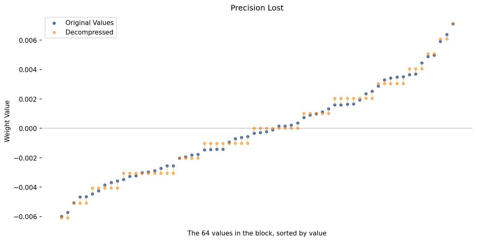
Not too bad!

Notice how the orange bars (the decompressed numbers) only take on a limited set of values–the possible values are the fifteen numbers from

For this block, we made use of 14 of the 15 possible values (count up the number of groups of orange bars to see this. The only value we didn’t use is -|max|).

That seems like a good sign–we’re making great use of the available precision. It’s like we’ve created a custom 4-bit data type that best represents these 64 numbers!

This is quantization. We’ve taken a continuous valued number and mapped it to a discrete set of values.

It worked particularly well here because our block did not contain any outlier values–that’s an important topic we’ll come back to.

First, though, let’s look at their custom NF4 data type to see how it improves on the above.

S4. Natural Float4 (“NF4”)

The far left and right ends of our example plot, where there are fewer values mapped, are a result of the normal distribution of the weight values.

Seems like we might be able to represent this data a little more accurately if we could have more distinct values close to zero–i.e., if the distribution of our 15 values better matched the distribution of our data.

That’s the idea behind the NF4 data type.

4.1. NF4 Values

The 4Q authors gathered statistics on a number of popular models and determined the values that would best match the overall distribution of neural network weights. These are hardcoded values defined by NF4 (from Appendix E, pg. 24 of the paper):

import numpy as np

# Hardcoded quantization values
nf4_values = np.array([-1.0, -0.6961928009986877, -0.5250730514526367,
                       -0.39491748809814453, -0.28444138169288635, -0.18477343022823334,
                       -0.09105003625154495, 0.0, 0.07958029955625534, 0.16093020141124725,
                        0.24611230194568634, 0.33791524171829224, 0.44070982933044434,
                        0.5626170039176941, 0.7229568362236023, 1.0])

print(nf4_values)

[-1.     -0.6962 -0.5251 -0.3949 -0.2844 -0.1848 -0.0911  0.      0.0796
  0.1609  0.2461  0.3379  0.4407  0.5626  0.723   1.    ]

This time, there are 16 of them… They call it an “asymmetric data type” because, in order to make use of all 16 values (but still have one of them be 0) they have 8 positive values, but only 7 negative.

# 7 negative values
print("There are {:} negative values:".format(len(nf4_values[0:7])))
print(nf4_values[0:7])

# 8th value is zero
print("\nThe 8th value is zero:")
print(nf4_values[7])

# 8 positive values
print("\nThere are {:} positive values:".format(len(nf4_values[8:16])))
print(nf4_values[8:16])

There are 7 negative values:
[-1.     -0.6962 -0.5251 -0.3949 -0.2844 -0.1848 -0.0911]

The 8th value is zero:
0.0

There are 8 positive values:
[0.0796 0.1609 0.2461 0.3379 0.4407 0.5626 0.723  1.    ]

I had ChatGPT help me generate a cute plot for visualizing them and their spacing (the code’s in the appendix).

It’s a little convoluted, but here’s how to look at it:

1. First, ignore the colors, and just look at the two number lines, and see how the placement of values differs.
2. Second, the colors show the size of the gap between each value and the next. For sevenths, it’s just solid blue because the interval is always just 1/7!.

A couple observations:

1. Because NF4 only has seven negative values but eight positive values, the negative values are a little further spread out (and lighter in color).
2. Comparing the two, I think you could summarize the difference as:
   • NF4 drops the ability to represent -6/7|max| and +6/7|max|.
   • This allows NF4 to squeeze three additional values (the third comes from using all 16!) bettwen the range -5/7 to 5/7.

Let’s re-run our compression-decompression example to see how things turn out when we use the NF4 values instead of uniform intervals of 1/7.

4.2. Applying NF4

Let’s compress and decompress our example block, but with the NF4 values instead of “sevenths”.

This time, I’ll define a function for the task. I generally try to avoid this in tutorials, since the purpose is learning (not developing), and functions obscure what’s going on. In this case, though, it will allow us to quickly run this same experiment with different blocks (which we’ll do in the next section on outliers).

import numpy as np


def run_4Q(block_values, use_nf4 = True):
    '''
    Compresses and decompresses `block_values` by applying 4-bit quantization.
    The purpose is to compare the values before and after in order to
    investigate the loss in precision.
    Set `use_nf4` to use the NF4 4-bit values, otherwise it uses sevenths.
    '''

    # ======== Rescale to -1 to +1 ========

    # Find the number with the highest absolute value.
    abs_max = np.max(np.abs(block_values))

    # Divide all of the numbers by it.
    scaled_values = block_values / abs_max

    # After rescaling, our values are much better aligned to the 4-bit values
    # (which also have the range -1 to +1)

    # ======== Choose 4-bit Data Type ========

    if use_nf4:
        # The NF4 datatype defines 16 hardcoded values.
        dtype_values =  np.array([
            -1.0, -0.6961928009986877, -0.5250730514526367,
            -0.39491748809814453, -0.28444138169288635, -0.18477343022823334,
            -0.09105003625154495, 0.0, 0.07958029955625534, 0.16093020141124725,
            0.24611230194568634, 0.33791524171829224, 0.44070982933044434,
            0.5626170039176941, 0.7229568362236023, 1.0], dtype='float16')
    else:
        # Uniformly spaced ("sevenths")
        dtype_values = np.linspace(-1, 1, 15, dtype='float16')

    # ======== Map to nearest 4-bit value ========
    # This mapping step is where the rounding error occurs.

    # Compressed representation of our values.
    compd_values = []

    # For each value...
    for i, scaled_val in enumerate(scaled_values):

        # Calculate the absolute difference between the current weight value
        # and all the 4-bit values
        diffs = np.abs(dtype_values - scaled_val)

        # Get the index of the closest matching number (the smallest difference)
        dtype_i = np.argmin(diffs)

        # Replace our weight value with the corresponding 4-bit number.
        compd_values.append(dtype_values[dtype_i])

    # Make it a numpy array for further math.
    compd_values = np.asarray(compd_values)

    #print(compd_values)

    # ======= Decompress ========

    # Decompress the values by multiplying them by the absolute maximum.
    decompd_values = compd_values * abs_max

    #print(decompd_values)

    return(decompd_values)

Side Note: I’ve dug through the actual bitsandbytes code for this, and it actually uses a decision tree to efficiently map the values! (in my code I simply used argmin). The source is here.

Now apply it to our block.

# Compress and decompress using NF4 as the intermediate representation.
decompd_values = run_4Q(block_values, use_nf4 = True)

This time, the possible values are (roughly):

I’ll also define a function for the scatter plot.

I added one feature–this will draw horizontal lines at each of the (15 or 16) possible values after running 4Q. This helps show how well our data fits to the available precision.

import numpy as np
import matplotlib.pyplot as plt

def plot_precision_loss(original_values, decompressed_values, use_nf4 = True):

    # ======== Plot Setup ========

    # Set global font size
    plt.rc('font', size=10)  # Adjust the font size as needed

    # Set the plot size
    plt.figure(
        figsize=(12, 6),
        dpi=150 # Increase quality if needed
    )

    # ======== Draw the possible values ========
    # We'll draw horizontal lines at each of the (15 or 16) possible values
    # that the data can take on after running 4Q.

    if use_nf4:
        # The NF4 datatype defines 16 hardcoded values.
        dtype_values =  np.array([
            -1.0, -0.6961928009986877, -0.5250730514526367,
            -0.39491748809814453, -0.28444138169288635, -0.18477343022823334,
            -0.09105003625154495, 0.0, 0.07958029955625534, 0.16093020141124725,
            0.24611230194568634, 0.33791524171829224, 0.44070982933044434,
            0.5626170039176941, 0.7229568362236023, 1.0], dtype='float16')
    else:
        # Uniformly spaced ("sevenths")
        dtype_values = np.linspace(-1, 1, 15, dtype='float16')

    # Find the number with the highest absolute value.
    abs_max = np.max(np.abs(original_values))

    # The data can now only take on a limited set of values, given by
    # the 4-bit data type and the abs_max of the input data.
    possible_values = dtype_values * abs_max

    # Draw horizontal lines at each of the possible decompressed values
    for val in possible_values:
        plt.axhline(
            y = val,
            color='orange',
            linestyle='--',
            linewidth=0.5)

    # Set x-axis at 0
    plt.axhline(0, color='grey', alpha=0.5, linewidth=1)

    # ======== Sort the values in ascending order ========

    # Get the indices that would sort the block array
    sorted_indices = np.argsort(original_values)

    # Sort both arrays based on the indices
    original_values = original_values[sorted_indices]
    decompressed_values = decompressed_values[sorted_indices]

    # ======== Plot the values before and after 4Q ========
    # We'll use two scatter plots.

    # This serves as the x axis values.
    val_indeces = np.arange(1, 65)

    # Colors for our two plots.
    grey_blue = (0.2980392156862745, 0.4470588235294118, 0.6901960784313725)
    dark_orange = (1.0, 0.5, 0.0)  # Darker orange color

    # Scatter plot for Original Values
    plt.scatter(
        x = val_indeces,
        y = original_values,
        color = grey_blue,
        s = 15, # Make the markers smaller
        label = 'Original Values'
    )

    # Scatter plot for Decompressed Values
    plt.scatter(
        x = val_indeces, # Just the numbers 1 - 64
        y = decompressed_values,
        color = dark_orange,
        alpha = 0.5, # Make it transparent so we can see overlap.
        label = 'Decompressed',
        s = 15, # Make the markers smaller
    )

    # ======== Connect the values ========
    # Plot vertical lines between each pair to help clarify which
    # belong together.

    # For each of the 64 values...
    for i in range(len(val_indeces)):
        # Plot a vertical line.
        plt.plot(
            # x values for the start and end points.
            [val_indeces[i], val_indeces[i]],

            # Corresponding y values for the start and end points.
            [original_values[i], decompressed_values[i]],

            # Line properties
            color = 'orange',
            alpha = 0.5,
            linewidth = 1
        )

    # ======== Plot vertical scale ========
    # Set the vertical "zoom" to include all possible values (even if they
    # aren't all used)
    y_min = -abs_max - 0.001
    y_max = abs_max + 0.001

    plt.ylim(y_min, y_max)

    # ======== Plot Styling ========

    # Label the plot
    plt.title('Precision Lost')
    plt.xlabel('The 64 values in the block, sorted by value')
    plt.ylabel('Weight Value')

    # Include the legend. Place it in the upper left corner of the plot, where
    # we know there won't be any data.
    plt.legend(loc='upper left')

    # Remove plot boundaries
    plt.gca().spines['top'].set_visible(False)
    plt.gca().spines['right'].set_visible(False)
    plt.gca().spines['left'].set_visible(False)
    plt.gca().spines['bottom'].set_visible(False)

    # Remove x-axis ticks and labels--these aren't meaningful in this context.
    plt.xticks([])

    plt.show()

plot_precision_loss(block_values, decompd_values, use_nf4 = True)

S5. Outliers

Overall, the precision of 4Q seems surprisingly good!

That’s rather remarkable given that the block of 64 numbers we grabbed from the weight matrix don’t actually have any relationship to one another! There’s nothing about “neighboring weights” that would suggest they should require similar compression.

What they do have in common, though, is that they all belong to that normal distribution that we plotted for the matrix.

That means that what we saw in our above example is pretty typical–our values are usually going to fall neatly within a well defined range (for example, 95% of the values we come across are going to fall within be within two standard deviations of the mean) and be spread relatively uniformly in that range.

Image taken from here

We’ve been avoiding the obvious question for long enough–what happens when there are outliers?!

Here’s what to know:

1. Outliers definitely hurt the quality of the results, since they expand the range we have to cover, leading to less precision.
2. The “absolute maximum rescaling” approach we’re using exacerbates this problem (“linear rescaling”, which we’ll look at, allocates things better).
3. Outliers are apparently very important values in neural network weights.
4. Because of this, the abs-max approach is actually preferable in this context.

Let’s look at these points in a little more detail.

5.1. Outlier Examples

Using the functions we defined earlier, let’s check out the compression loss for a couple of blocks containing outliers.

I scanned through the 256K blocks in our example matrix to look for examples.

• 1st Example - I only had to scan through to 20th block in order to find one containing a value more than 3 standard deviations from 0.

• 2nd Example - I also searched for a more extreme outlier, greater than 0.06 (the largest outlier in the matrix is 0.0698) and found one at block 36,384.

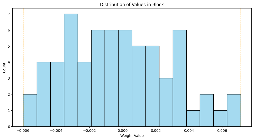
Here are the values for the first example.

outlier_block = np.asarray([
  3.66210938e-03,  6.63757324e-04, -6.04248047e-03,  1.09863281e-02,
 -1.87683105e-03, -3.07559967e-05, -3.77655029e-04, -1.65557861e-03,
 -1.83105469e-03,  5.24902344e-03,  4.02832031e-03,  4.08935547e-03,
  6.10351562e-03, -3.06701660e-03,  3.96728516e-03,  1.90734863e-03,
 -2.07519531e-03,  3.34167480e-03,  3.17382812e-03,  2.71606445e-03,
  3.25012207e-03, -7.93457031e-04, -3.09753418e-03,  2.86865234e-03,
  1.14440918e-03,  1.69372559e-03,  4.02832031e-03, -4.25338745e-04,
 -6.63757324e-04, -7.93457031e-04,  1.32751465e-03, -1.31130219e-05,
 -2.45666504e-03,  1.06048584e-03,  1.99890137e-03, -7.53784180e-03,
  2.80761719e-03, -2.28881836e-03, -7.32421875e-03, -3.89099121e-03,
  2.04086304e-04, -2.34985352e-03, -6.40869141e-03, -5.22613525e-04,
  6.75201416e-04,  3.82995605e-03, -2.16674805e-03,  6.10351562e-03,
 -2.34985352e-03,  1.95312500e-03, -2.51770020e-04, -4.21142578e-03,
 -3.99780273e-03, -8.16345215e-04, -2.68936157e-04, -4.36401367e-03,
 -5.88893890e-05, -6.07299805e-03, -2.05993652e-03,  1.10149384e-04,
  1.13487244e-04, -3.69262695e-03,  4.02832031e-03,  2.59399414e-03])

min_value = min(outlier_block)
max_value = max(outlier_block)

print(f"Min: {min_value}")
print(f"Max:  {max_value}")

Min: -0.0075378418
Max:  0.0109863281

Let’s plot the distribution of the values, and we’ll see our outlier.

import seaborn as sns
import matplotlib.pyplot as plt

# Plot distribution using seaborn

# Set the aspect ratio
plt.figure(figsize=(12, 6))

# Plot as a histogram with 500 bins.
hist = sns.histplot(outlier_block, bins=16, kde=False, color='skyblue')

# Draw vertical lines at the min and max
plt.axvline(x = min_value, color='orange', linestyle='--', linewidth=1)
plt.axvline(x = max_value, color='orange', linestyle='--', linewidth=1)

# Label the plot
plt.title('Distribution of Values in Block')
plt.xlabel('Weight Value')
plt.ylabel('Count')

# Display
plt.show()

Here’s the distribution of values in the block–the outlier value is at ~0.011.

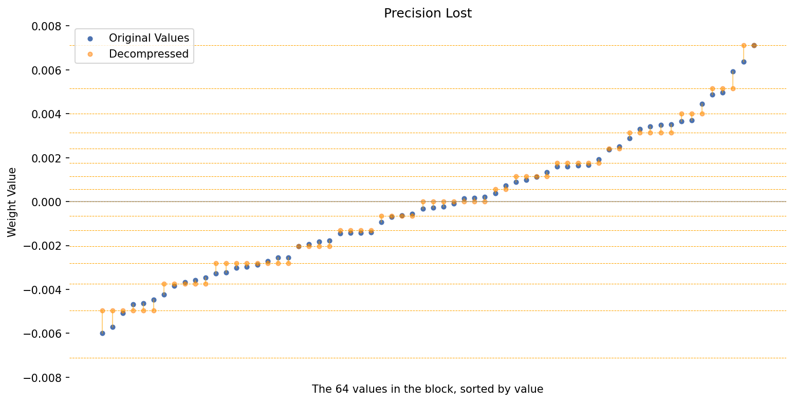
Next, we can use the functions we defined earlier to run the 4Q algorithm and plot the values “before and after”.

If you check each of the horizontal lines, you’ll notice that we’re still using 14 out of 16 possible values, though the values on either end aren’t being used much.

# Run 4-bit quantization
decompd_values = run_4Q(
    block_values = outlier_block,
    use_nf4 = True
)

# Generate a plot to visualize the loss in precision.
plot_precision_loss(
    original_values = outlier_block,
    decompressed_values = decompd_values
)

Extreme outlier

Here are the values for our second example, with an even bigger outlier.

outlier_block = np.asarray([
 -0.00282288, -0.00631714,  0.00364685,  0.00216675,  0.00314331, -0.00033379,
  0.00254822, -0.00093079, -0.00212097, -0.00231934,  0.00115967,  0.00457764,
  0.00674438,  0.00585938, -0.00271606,  0.00152588,  0.00268555,  0.00390625,
  0.00191498,  0.00769043,  0.00021267, -0.00445557,  0.06298828, -0.00173187,
  0.0010376 , -0.00445557, -0.00415039,  0.0045166 ,  0.00415039,  0.00488281,
  0.01965332,  0.00221252, -0.00674438,  0.00285339,  0.00570679,  0.02050781,
  0.00349426, -0.00121307, -0.00064087, -0.00497437, -0.00549316, -0.00534058,
 -0.00159454,  0.00146484, -0.00036049,  0.00092316,  0.00650024, -0.00035095,
 -0.00567627,  0.00482178, -0.00012779, -0.00071335, -0.00222778, -0.00476074,
  0.00141144, -0.00059128,  0.00411987,  0.0019989 ,  0.00318909,  0.00018501,
 -0.00161743,  0.00291443, -0.00177765, -0.00379944])

min_value = min(outlier_block)
max_value = max(outlier_block)

print(f"Min: {min_value}")
print(f"Max:  {max_value}")

# TODO - Print "Range", then "Smallest" and "Biggest" values.

Min: -0.00674438
Max:  0.06298828

import seaborn as sns
import matplotlib.pyplot as plt

# Plot distribution using seaborn

# Set the aspect ratio
plt.figure(figsize=(12, 6))

# Plot as a histogram with 500 bins.
hist = sns.histplot(outlier_block, bins=16, kde=False, color='skyblue')

# Draw vertical lines at the min and max
plt.axvline(x = min_value, color='orange', linestyle='--', linewidth=1)
plt.axvline(x = max_value, color='orange', linestyle='--', linewidth=1)

# Label the plot
plt.title('Distribution of Values in Block')
plt.xlabel('Weight Value')
plt.ylabel('Count')

# Display
plt.show()

This is pretty extreme! And our plot below shows that 60 of the 64 values in the block map to just 3 numbers–mostly to zero!

# Run 4-bit quantization
decompd_values = run_4Q(
    block_values = outlier_block,
    use_nf4 = True
)

# Generate a plot to visualize the loss in precision.
plot_precision_loss(
    original_values = outlier_block,
    decompressed_values = decompd_values
)

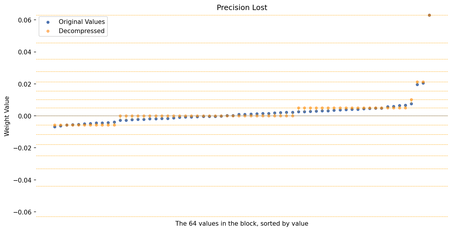
There’s a problem with our plot–the y-axis range on previous plots was about -0.01 to +0.01, but here we’ve zoomed out to -0.06 to +0.06, and so the sizes of the differences aren’t comparable.

We could zoom in on -0.01 to +0.01 to look at the change in those values in a comparable way.

However, this also points to a more general problem with trying to plot the precision loss…

The significance of the error is relative to the magnitude of the original value.

For example, one of the values in this example is about −0.000013.

A change of 0.00001 to this value is massive (about 80%), where as rounding the value 0.008 by that amount is negligible (about 0.1%).

In other words, 4Q has massive precision loss for “tiny values”. So why does it work?

5.2. Outliers & Zeros

The QLoRA paper points to research showing that the outlier values in neural network weights are the most important.

This makes intuitive sense–larger weight values mean a higher magnitude dot product and a higher activation value.

Though it’s not discussed in the paper, I think it also makes intuitive sense that weight values close to zero can be ignored. They have a neglible impact on the dot product, and so very little influence over the behavior of the network.

It makes sense to me, then, that it’s safe to round “tiny” weight values to zero.

I think this is a key insight into why 4Q works. When allocating precision to a floating point data type, a key consideration is how tiny of values it can represent. 4Q does a bad job at preserving these values, and that doesn’t seem to matter for neural networks!

S7. Conclusion

Here are what I see as the key take-aways:

1. A 16-bit model with 4-bit quantization (“4Q”) applied is still just a 16-bit model, not 4-bit.
   • 4Q is just a compression technique for storing the model with less GPU memory.
   • It does not do anything else to help with the compute or memory consumption required for running or fine-tuning a model.
2. 4Q does not achieve a full 4x reduction in memory use.
   • Like any compression technique, there is additional metadata stored that’s required for recovering the original values, making the reduction more like, e.g., 3.76x.
3. 4Q cannot be used for pre-training the next GPT or LLaMA.
   • It freezes the model weights.
   • It can only be used for fine-tuning, by adding-on additional trainable weights with LoRA.
4. For every block of 64 values in a matrix, 4Q effectively “chooses” 16 ~normally distributed values to best represent all of the values in that block.
5. It works by leveraging three key aspects of neural network weights:
   1. Weight values are normally distributed.
   2. Large weight values are the most important (and 4Q preserves large weight values with high precision).
   3. Tiny weight values are irrelevant (and 4Q just rounds these to zero).

Appendix

Discord

Questions or feedback? Leave a comment below, or better yet join us on our discord!

References

I built my initial understanding of QLoRA on this blog post by Dilli Prasad Amur, and some from this post by Sebastian Raschka. Ultimately I had to dig into the CUDA kernels to confirm my understanding.

Diving Deeper

Members have access to a video walkthrough, review notes, and further insights–join today!