The Inner Workings of DeepSeek-V3

I was curious to dig in to these DeepSeek models that have been making waves and breaking the stock market these past couple weeks (since DeepSeek-R1 was announced in late January ‘25).

i. Architecture of a Reasoning Model

I dug into the details of R1’s model architecture, thinking it might hold the answers to how reasoning works…

I figured out pretty quickly that it doesn’t.

(As I covered in my previous post, it’s really nothing more than a prompt telling the model to think before answering!)

Reasoning models are created by taking a base model like GPT-4o or DeepSeek-V3, and then training it to generate reasoning tokens in between <think> tags before providing its answer.

What this means is that R1 and V3 are the same underlying model, with the same code used to run either one, just with different weights.

ii. Efficient Training & Inference

While V3’s architecture may not hold the key to how reasoning works, it seems worth studying given that:

1. V3 and R1 are apparently competitive with their OpenAI counterparts (4o and o1).
2. V3 was trained at a lower cost than other “frontier models” like Llama 3 and GPT-4o.

I tend to be most curious about any changes to the internals of the Transformer, so this tutorial is going to focus on the two modifications that DeepSeek made:

• Multi-Head Latent Attention (MLA) - A technique for reducing the cost of inferencing a model (i.e., in production, how much it costs to answer user prompts).
• Mixture of Experts (MoE) - A technique for greatly reducing the number of calculations required to run the model, which is a big part of what reduced their training costs.

For Further Research

I want to point out a few other notable details which I haven’t covered in this tutorial, but could be worth diving into further:

1. A good chunk of the V3 paper addresses the hardware optimization they did to improve training efficiency.
   • I’d be curious to know more about how proprietary or not this work is, and whether it can be leveraged effectively for future models, or was highly tailored to their setup.
2. They utilized a novel training objective where, instead of predicting just the next token, they predict the next two tokens. They named this Multi-Token Prediction (MTP).
   • This technique is about extracting more training information per token in your dataset. Not sure whether that translates to lower cost training, higher performing models, or both.
3. Their R1 paper is all about their training pipeline for creating a high-performing reasoning model.
   • My understanding is that, if you want to know how they managed to produce a competitive reasoning model, the answer is in the details of the training process.

Maybe I’ll get to explore those later, but for now, let’s look inside V3!

▂▂▂▂▂▂▂▂▂▂▂▂

S1. Multi-Head Latent Attention (MLA)

MLA primarily about reducing the amount of $$$ it costs to serve an LLM.

DeepSeek also claims that MLA outperforms standard Multi-Head Attention, which is fascinating! I’m curious to see if other companies will find the same and begin using it.

MLA reduces inference costs by reducing memory requirements.

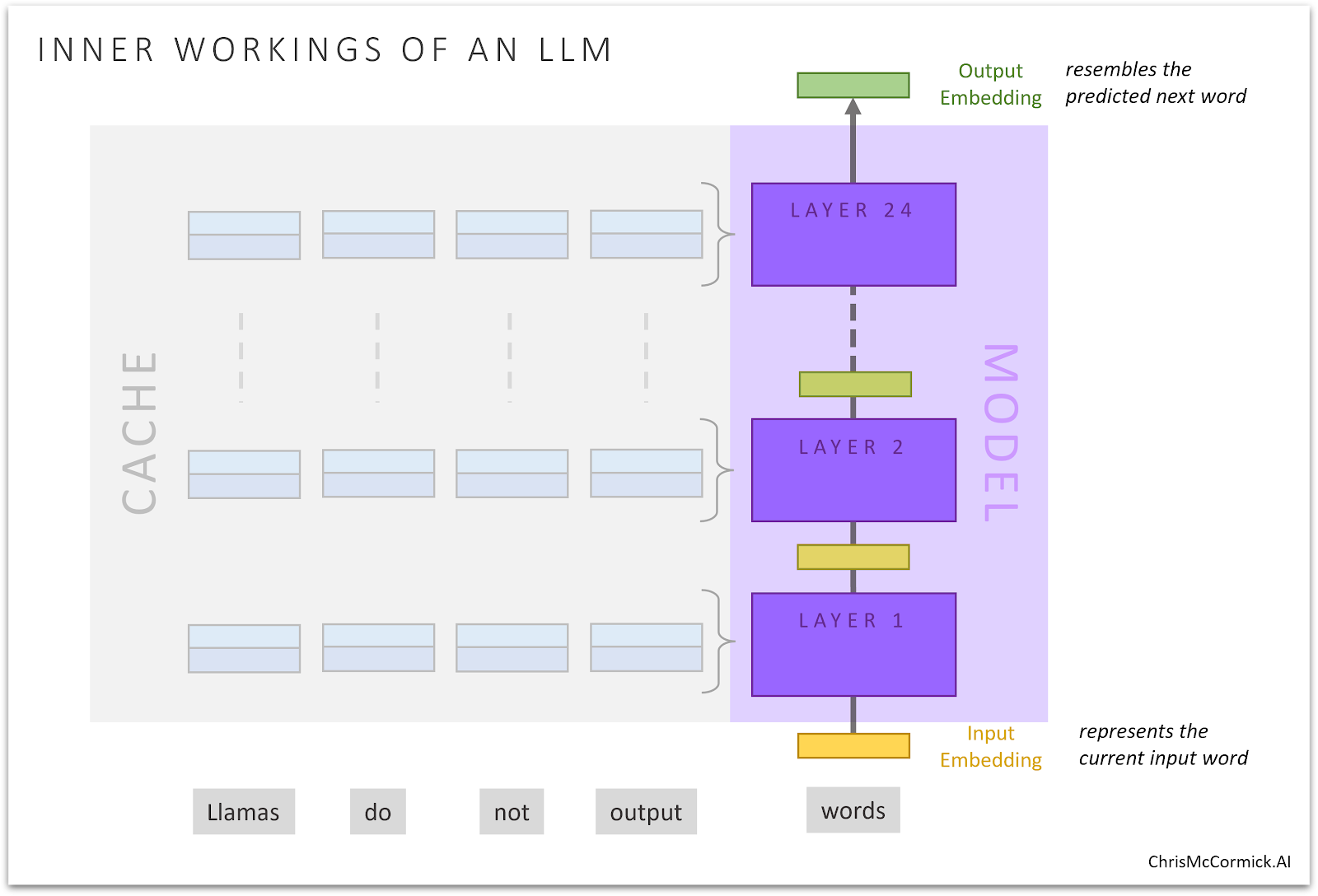
1.1. Memory Required for Caching

Something I hadn’t considered or studied before was the staggering amount of memory required to run inference on these huge models (with large embeddings and lots of layers) for long sequence lengths.

The problem comes from the practice of caching information about prior tokens.

A decoder model like DeepSeek-V3 processes one token at a time, and the Attention mechanism allows it to look back over the previous tokens and pull relevant information from them.

After processing a token, the model caches the data needed for future tokens to attend back to it. Specifically, it hangs onto the “Key” and “Value” vectors for every word, and does so at every layer.

Aside: What are key and value vectors? We use the “key” vectors for past tokens to determine whether and how to attend to them. For the tokens that we want to attend to, we pull information about them from their “value” vectors.

In the below illustration, the cached key and value vectors are represented by the blue rectangles. We’re caching 2 vectors per token, per layer.

Memory Required by MHA

To understand just how big of a concern this can be, let’s look at how much cache memory DeepSeek-V3 would need if it had used standard Multi-Head Attention (MHA).

V3 has 61 layers, an embedding size of 7,168 (7k), and supports a maximum sequence length of 128k tokens.

By the time we got to the 128k’th token (i.e., the very last one) in that window, here’s how much memory our cache would be consuming:

Staggering!

Other current giant models, like Mistral and Llama, had to contend with the same issue as well, of course. They used a technique called “Grouped-Query Attention” (GQA).

MLA requires even less memory than GQA (and apparently performs better as well??).

1.2. KV Compression

The main difference in MLA is that it decomposes the Key and Value projection matrices into an “A” and “B”, similar to LoRA.

Standard Multi-Head Attention uses (typically square) matrices to perform the projections onto “Key Space” and “Value Space”

Multi-Head Latent Attention replaces the blue and green matrices above with a kind of compress-then-decompress step.

Instead of a single “Key” projection matrix you get two matrices:

1. A “down” matrix that projects the token embedding down to a smaller dimension (512), and then
2. An “up” matrix that projects it back up to the larger dimension.

Compress, then decompress.

Normally, this would translate into 4 matrices (key down and up, value down and up), but MLA uses a single, shared down matrix for both the keys and the values.

(They refer to this technique as “joint KV compression”, FYI)

So in the below illustration, we have:

1. A single “KV Down” matrix for compressing the token embedding down to a vector with only 512 dimensions, which they call the “latent”.
2. “Key Up” and “Value Up” matrices for projecting the latent back up into those respective spaces.

Memory Savings

The compressed version of the token embedding–the 512-value latent–is the only vector cached for each token.

That means it reduces the total storage for a token from 14k values down to just 512!

That’s 28x smaller, bringing the maximum KV cache size from 213.5 GB all the way down to 7.6 GB.

Note: DeepSeek-V3 has 128 attention heads with 128 values each. It uses an embedding size of 7k, but the key and value vectors are actually 16k.

How does it work for their to be a mismatch? It’s the job of the Attention Output matrix to combine and project the results back into the token embedding space.

Challenges

I think that’s a good general intro to MLA, but there are a couple key pieces required to actually make this technique work which I’ll have to come back to in a follow-up post.

1.3. Cost of Decompression

Problem #1: Less Memory, More Compute?

The reason we cache the key and value vectors is to avoid having to recalculate them for every new token–to avoid having to redo the K and V projections over and over.

We’ve saved a lot of cache memory here, but we’re back to having to recompute the key and value vectors for every new token!

It’s less compute than before (since our latent is only length 512), but still unacceptable.

However, through some black magic–oops, I mean, basic algebra–they were able to avoid the decompression step.

Specifically:

1. Decompressing the Key (“Key Up”) can be absorbed into the Query calculation, and
2. Decompressing the Value (“Value Up”) can be absorbed into the Attention Output matrix.

Pretty fascinating to me that that would work–I still need to go work through the math to see it better.

1.4. Position Encoding

Problem #2: RoPE

There’s still one more problem…

RoPE (Rotational Position Embeddings) is a technique applied to the query and key vectors which encodes position information into them so that the model actually gets to know the word order.

Apparently this whole MLA approach, as we’ve defined it so far, breaks the RoPE math.

“Decoupled RoPE Embeddings”

This RoPE issue is another place where I have to point out that, though I know a lot of the details now, I still need to dig a bit deeper before I can claim to fully understand it. Sorry. 😕

Here’s what they do differently to fix it: Instead of applying RoPE to the keys and values directly, that information gets concatenated to them.

It’s kept separate from the latent, and then gets brought back in as part of the attention scoring calculation.

You can see the concatenation step illustrated in their architecture diagram below.

The third row from the bottom shows those separate “RoPE embedding” calculations.

1.5. Impact on Performance

Efficiency and Performance?

A bizarre (but exciting?) detail is that they claim that, unlike rather than compromising the performance of the model for the sake of inference cost (which is apparently, MLA actually just plain works better than standard Multi-Headed Attention! Pretty crazy!

Multi-Head Latent Attention (MLA) was introduced by DeepSeek in their V2 model in June 2024, here. Here is their introduction of MLA in the intro of their V2 paper. (I’ve kept their text verbatim, but added bullets and emphasis.)

In the context of attention mechanisms, the Key-Value (KV) cache of the Multi-Head Attention (MHA) (Vaswani et al., 2017) poses a significant obstacle to the inference efficiency of LLMs.

• Various approaches have been explored to address this issue, including
  • Grouped-Query Attention (GQA) (Ainslie et al., 2023) and
  • Multi-Query Attention (MQA) (Shazeer, 2019).
• However, these methods often compromise performance in their attempt to reduce the KV cache.

In order to achieve the best of both worlds, we introduce MLA, an attention mechanism

• equipped with low-rank key-value joint compression.
• Empirically, MLA achieves superior performance compared with MHA,
• and meanwhile significantly reduces the KV cache during inference,
  • thus boosting the inference efficiency.

Nick once pointed out to me that the best test of one of these new ideas is whether or not they get adopted in the next generation of “frontier” models. I’m eager to find out!

Another aspect of V3 that differs from the standard Transformer is the “Mixture of Experts” strategy used in the Feed Forward Networks. This isn’t a new idea from DeepSeek, but they seem to have used it quite successfully, so let’s check it out.

▂▂▂▂▂▂▂▂▂▂▂▂

S2. Mixture of Experts (MoE)

MoE is about reducing the amount of $$$ required to train an LLM by reducing the number of gradients we have to calculate on the Feed Forward Networks (FFNs).

Side Note: I wonder how you decide whether to frame something as “train a model for less” vs. “make it feasible to train bigger, better models?”

FFN Terminology

A standard Transformer layer consists of an Attention block and then a (big!) Feed-Forward Network (FFN). Most of the parameters in an LLM actually reside in these FFNs.

An FFN has an “intermediate layer” and an “output layer”.

Llama 3, as an example, uses an embedding size of 16,384, and the intermediate layer of its FFN is a matrix that’s [16,384 x 53,248] i.e., [16k x 52k]. The output layer is the same size, transposed.

(For anyone counting, that’s 1.66B parameters!)

I like to apply the language of Multi-Layer Perceptrons (MLPs) and the concept of a “neuron”.

Each one of those 52k column vectors is considered a neuron, and so Llama 3 uses an FFN with 52k neurons in its transformer layers.

An Even Bigger FFN?

In V3, they replace the standard, huge FFN with… an even bigger one.

The FFN in a V3 layer has 512k neurons! 😱 Roughly ten times bigger than an FFN in Llama 3.

We seem to have gotten off track–weren’t we talking about reducing the cost of training the model?

The key is that a given token only gets sent to 16k of those neurons, so we effectively only have to calculate the gradients on weight matrices of size [7k x 16k] instead of [7k x 512k].

2.1. Clustering Neurons

To do this, they break that big collection of 512k neurons into 256 clusters of 2k neurons each.

And before sending a token in, they compare it to the 256 “centroids” (one per cluster), and only send it to the top 8 closest ones.

8 clusters of 2k neurons each means, again, that only 16k neurons are actually evaluated for a given token.

The terminology used for one of these clusters is an “expert”. I’m guessing because the 2k neurons are presumably related (I think they need to be in order for the routing math to work well), so maybe the cluster has an underlying “area of expertise”.

Routing

Below is their architecture diagram for the Mixture of Experts component.

Some things to note:

• Number of Experts:
  • There is actually only 1 shared expert (the green boxes).
  • There are 256 routed experts (blue boxes).
    • A token goes through only the top 8 of these.
• Expert Size:
  • The DeepSeek-V3 embedding size is 7k.
  • The hidden layer of each expert has 2k neurons.

2.2. Double-Gating

The 512K neurons in an MoE layer are actually gated twice…

Each expert is an MLP with 2,048 neurons and uses SWiGLU. This means that when a token is sent an expert, a second round of gating occurs to determine which of those 2k neurons it (effectively) sees.

The difference is that, in the routing step, we literally only do the calculations for the 8 selected clusters–all the other neuron activations are directly set to 0.0.

In contrast, with SWiGLU, even though we are “gating” (many of?) the 2k neurons, we’re still doing the full matrix multiplications for all 2k neurons.

(Another difference–the “Swish” part of SWiGLU makes it a softer gate that doesn’t necessarily return precisely 0.0).

Memory Access

Why not just skip the whole “clusters” / “experts” bit and just take the top 8x2k = 16k neurons from the FFN?

1. It would mean comparing the input to 512k gate vectors instead of just 256 cluster centroids.
2. Once we found those top 16k, it’d mean a whole lot of random access to pull together their weights.

A lot of Wasted Math

This highlights what seems to me like a very interesting aspect of the Transformer architecture in general.

We do (A) a lot math to determine that (B) a lot of the other math we did wasn’t necessary–“don’t attend to those tokens”, or “don’t incorporate information from those neurons”.

Lots of expensive dot-products end up reduced to zero (or close to it).

MoE exploits this fact to cut down the amount of (B) that we do, and (at least partially) avoids the challenge of sparse matrix multiplication by encouraging the model to group together neurons that are likely to fire together.

It makes me wonder–could the same clustering technique be applied to the attention heads? 🤔

▂▂▂▂▂▂▂▂▂▂▂▂

Conclusion

It’s hard to write a conclusion here. I feel like I have more interesting questions than answers.

Multi-Head Latent Attention

This mainly seems to get emphasized as a technique for reducing the KV cache size.

But I’m more interested in its implications on Attention in general.

• Apparently only 512 features are enough to be able to produce effective Key and Value vectors?
• Once learned, can the Value projection matrix just be folded in to the Output matrix??
  • And the Query and Key projections merged in some similar way?

Mixture of Experts

This is mainly emphasized as a way to reduce training cost by reducing the number of activating parameters.

That makes sense. But could it also be framed as an opportunity to scale up? To wildly increase the capacity of our LLMs, without paying the cost?

The whole concept of doing a “hierarchical search” to find the right neurons gets my gears turning, too. Where else could we apply that concept? Could we cluster or index the cached keys to reduce the cost of attention scoring?

Fun stuff.