Patterns and Messages - Part 1 - The Missing Subscript

In this post, we’ll look at how a tiny bit of algebra suddenly opens up a wealth of insight.

I want to clarify up front that none of the “rearranging” that I do in this post is intended to change how we implement Attention. It’s about exposing underlying operations that are already there–we just haven’t noticed them because of the (important!) emphasis we place on finding computationally efficient algorithms.

Let’s see what happens when we prioritize conceptual clarity over GPU efficiency!

by Chris McCormick

Contents

• Contents
• The Hidden Structure in $W_O$
• $W^O_i$
• Output of a Head
• Value-Output Relationship
• Conclusion
• Appendix: Working Back to the Implementation

The Hidden Structure in $W_O$

When we write out Transformer attention, the final step is to recombine the output of the heads using the matrix $W_O$:

The concatenation step allows us to perform a single, large matrix multiplication in order to combine the results of the heads and project them back up to the same space as the input embedding (the “model space”).

I assume that’s a good move computationally, but it obscures important insights about what is actually going on in the attention math.

$W^O_i$

We don’t call it out in the equations, but inside of $W_O$ are actually independent, per-head output matrices, $W^O_i$. They are implicitly concatenated together and stored as one large matrix.

We don’t actually perform that second concatenation, but you could say it’s implied.

Concatenation is a bit of a bizarre operation for linear algebra–the resulting behavior is different than my normal intuition about what happens in a matrix multiply.

Typically, we’re multiplying every vector in one matrix against every vector in the other–i.e., all of the “items” in A interact with all of the ones in B. But it’s different when you stack matrices like this.

The values in $\text{head}1$ _only get multiplied against the values in their corresponding output matrix, $W^O_1$. They don’t see any of the other parameters.

The effect is the same as multiplying each of the corresponding smaller matrices against each other, and then summing the result:

Seeing it broken out like this was surprising to me, because it highlights the fact that each head is actually producing an independent output embedding, and then these are getting summed together (without any weighting) to produce the end result.

On the left is the original illustration from Attention is All You Need, but I’ve modified it to include the names of the weight matrices, and to highlight the implied concatenation.

On the right is an alternative version which is mathematically equivalent.

It’s not as computationally efficient as the concatenation approach, so it’s not how we implement it in practice, but it does make it a lot easier to explain the behavior of an attention head.

We can illustrate and explain the full behavior of a head without any reference to the concept of their being multiple heads.

The explanation for Multihead Attention then becomes, at least conceptually:

Every layer has a number of these heads running in parallel, and we sum their results.

Pretty straightforward!

The concatenation operation becomes “a modification we do to run better on a GPU”, and can be discussed separately.

Output of a Head

Side Note: From here on, I’m going to switch to talking about having a single input embedding (our query) and a sequence of tokens to attend to (our keys).

The fact that we can process multiple queries at once is another detail that’s important for computational efficiency, but distracting for thinking more conceptually about how things work.

We have nice intuitions about what the attention scoring part of a head does–we’ve demonstrated that the heads can identify semantic and syntactic relationships between words. It’s figuring out “what words to pay attention to”.

Breaking apart the output matrix has helped me think more clearly, though, about what a head actually does on the output.

We typically have two things that we might call the “output” of attention.

Output of “Attention”

The original equations define $\text{Attention}$ with the below equation, and later authors have adopted the variable $z$ for this step.

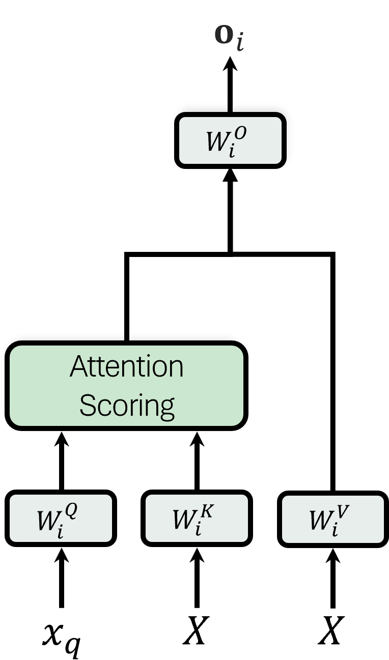
For a given input vector (and its query vector, $q_i$), the output of $\text{Attention}$ for head $i$ is:

$z_i$ is in the low-dimensional value space, $d_v$, making it harder to interpret.

Output of “MultiHead”

The other item we have is the result of $\text{MultiHead}$, which is given the variable $o$.

This is the output after combining all of the heads:

$o_t$ is in model space, $d_\text{model}$, which is cool for interpretability. But it combines all of the heads into one embedding, so it’s not really clear how each head contributes.

Output of a Head!

After removing the concatenation step and breaking apart the heads, we can look at it with a little more granularity.

Each head is actually outputting its own independent embedding:

Now for a given query, we can retrieve an output vector (in model space) to see what each head is returning!

This $o_i$ embedding never actually “exists” in the code, because the full-size $W_O$ step takes care of both computing the $o_i$ vectors and summing them together into a single $o_t$ in one big step.

But again–it’s definitely there!

Now we can explain the output of attention as:

Each head produces a separate, full-size embedding (not a value vector!) which represents its overal contribution to the attention output.

That’s a pretty cool insight, and something we should be able to exploit in investigating how the attention outputs impact the model.

This modification to the equations in turn allows for another change which helps clarify the roles of the Value and Output matrices.

Value-Output Relationship

Many illustrations of Attention follow the original in having the queries, keys, and values all pointing into an “Attention” block.

I find this a little confusing, because the word “attention” emphasizes the part of the process which scores the tokens–the multiplication of query and keys to determine which tokens to focus on.

The value vectors, though–they’re a part of the overall process, sure, but they have more to do with the modifications to the embedding that we’re going to make.

It feels like the process ought to be split out to separate the attention scoring from the embedding update.

Looking around online, there are definitely good illustrations out there which make this separation.

$\alpha_i$ is a square matrix of attention scores between every token, $T \times T$.

$V_i$ contains our tokens projected down into the small space of $\text{head}_i$, with size $T \times d_v$.

The standard equation for getting the output from those two things is:

But we can conceptualize it better by splitting this into:

And now we’ve stumbled into another way in which the computationally efficient definition has been obscuring something valuable.

Notice how the first form of the equation enforces a sequence of operations–the attention scores must be applied to the values first.

The second form lets us change the order, and compute the Output projections before applying the scores.

This creates a clean division of the two processes in attention:

1. The Query-Key process is for calculating the attention scores,
2. The Value-Output process is for producing the updates to make to the input.

Those updates are weighted by the attention scores and summed together to produce the “full-size” output (i.e., the same vector length as the tokens) of a single head.

Conclusion

We often view Attention as a monolithic process, where we focus on the full multi-head representation instead of examining the behavior per head. The equations define per-head operations, yet our tendency is to pull back and look at large matrix multiplications over all heads at once.

This stems from how the scoring and output projections are applied, but by making two (mathematically equivalent) tweaks to the equations:

• Change the ‘Concat’ to a sum
• Re-project the value before applying the scores

We can create a clearer picture of Attention for ourselves which better highlights two valuable pieces of intuition:

1. The multiple heads are independent and cleanly separable, and
2. The Query-Key and Value-Output processes are independent and cleanly separable as well.

This formulation should benefit new learners as well, provided that we then explain how this simpler form gets refactored for GPU efficiency.

In the next post, we’ll look at a more substantial change to the equations which can further improve our mental model–we’ll see how the pairs $W^Q_i, W^K_i$ and $W^V_i, W^O_i$ can be viewed as low rank decompositions of two larger matrices.

Appendix: Working Back to the Implementation

I found it informative to think through the steps for turning the more conceptual equations back into their GPU implementation form.

To make all of this more efficient on the GPU, we:

1. Concatenate the per-head attention matrices into $W^Q, W^K, W^V,$ and $W^O$ for matrix multiplication efficiency.
   • (We might also point out that the first three are then further concatenated into a single matrix?)
2. After projection, we need to recover the per-head queries, keys, and values by splitting the matrices back apart.
   • (If we continued in matrix form then the queries from all heads would be multiplied with the keys from all heads).
3. To apply $W^O$ efficiently, we:
   • Re-order the terms to apply the scores to the values first (i.e., compute the weighted sum of the value vectors to reduce them to a single, per-head $z_i$ vector), then
   • Concatenate the $z_i$ vectors from the different heads, and
   • Multiply the result against the concatenated $W^O_i$ matrices, which both
     • Re-projects them to the model space, and
     • Sums together the output of each head.

I’d like to come back to this at some point and add the full set of equations for both formulations. In particular, I think the “GPU form” ought to be explicit about the concatenating and splitting of the QKV matrices.