Patterns and Messages - Part 2 - Token Communication

In the previous post, we looked at how our tendency to think of Attention in terms of large matrix multiplications obscures some key insights, and we rolled back the GPU optimizations in order to reveal them (recapped in the next section).

In this post, we’ll continue this process of reformulating Attention in a way that’s mathematically equivalent to the original, but emphasizes conceptual clarity over GPU efficiency.

Specifically:

1. The $W^V_i, W^O_i$ matrix pairs can be viewed as low rank decompositions of a larger matrix $W^{VO}_i$, and I’ll motivate my proposed naming of “messages”.
2. The $W^Q_i, W^K_i$ matrix pairs can be viewed as low rank decompositions of a larger matrix, $W^{QK}_i$, and I’ll motivate my proposed naming of “patterns”.

by Chris McCormick

Contents

• Contents
• Query-Key and Value-Output
• Token Messages
• Token Patterns
• Pattern-Message Attention
  • Step 1: Cache a Message
  • Step 2: Attention Scoring
  • Step 3: Aggregate Messages
• Decomposing
• Conclusion

Query-Key and Value-Output

To recap the prior post:

We saw how the Output matrix is actually applied per head, and that the multiple heads are independent and cleanly separable.

This in turn highlights that the Output matrix is not a final step applied over the entire Attention process, but rather that the per-head Query-Key and Value-Output matrices belong to two independent processes.

This change makes it apparent that $XW^V_iW^O_i$ forms a linear operation, and that we could fold $W^V_i$ and $W^O_i$ together.

Should we actually merge them?

Keeping them decomposed is a deliberate choice, though. This decomposition:

1. Creates a bottleneck, encouraging the model to identify the salient features of the input.
2. Is computationally more efficient than the merged form.

For example, let’s say we have an embedding size of 4,096 and a head size of 128.

The projection $xW^{VO}_i$ requires 16M multiply-accumulate operations whereas $xW^V_iW^O_i$ only requires 1M.

Conceptual Value

There are benefits to thinking about Attention in this way, though.

• It defines a more fundamental form of what is happening in Attention.
• It emphasizes the decomposition as merely a design choice, which we could choose to approach differently.
• It lets us choose a single metaphor to describe the process, making it easier to learn and remember.

Token Messages

While $W^{VO}_i$ is a very logical name for the matrix, it doesn’t give us a name for the projected result of $XW^{VO}_i$. The result is “the per-head, weighted value vectors of the context vectors $X$, reprojected into model space.”

I think there’s a great opportunity here to define a new metaphor for improving our mental model of Attention.

The language in the Transformer Circuits framework includes significant communication terminology, and Graph Neural Networks already have a name for these vectors that we can use: “messages”.

This captures the idea that Attention is the mechanism by which tokens send and receive information from one another.

Also, because of the strong overlap between Transformers and Graph Neural Network architecture, “messages” has already been used by other authors to refer to the value vectors. We could say that we’re extending this to the reprojected values.

Extraction vs. Communication

I also appreciate that this language suggests a different direction of information flow from “attention”, which I feel has the implication that this is a process of the input vector choosing and extracting information from the context that it deems relevant to itself.

Separating the Query-Key and Value-Output processes makes it particularly clear that the input / query vector isn’t directly involved in the creation of the messages (except its own). It feels fair to say then that the messages are created by the context vectors as opposed to extracted from them.

Also, it seems possible that some messages have less to do with influencing the prediction for the current input token, and instead are part of a more complex behavior intended primarily to influence future tokens.

That would suggest an interpreation of the context tokens deciding whether (and how strongly) to communicate their message via the current input vector.

“Messages” then gives us language to view things from this alternate perspective.

Token Patterns

While the “existence” of $W^{VO}_i$ seemed quite apparent after separating the math for the heads, it wasn’t as obvious to me that $x W^Q_i \times XW^{K’}_i$ could be refactored in the same way or that there was any reason to.

It seemed clear that we need to extract patterns, unique to each head, from both the input vector and the context vectors in order to compare them and calculate attention scores. Both $W^Q_i$ and $W^K_i$ seemed fundamentally necessary.

That’s incorrect, though, and there’s definitely insight to be gained from thinking in terms of a merged $W^{QK}_i$ matrix.

Refactoring Query-Key

To merge these matrices, we re-arrange the terms into:

$xW^Q_iW^{K’}_iX^{‘}$

Which becomes

$xW^P_iX^{‘}$

We project a word vector onto $W^P_i$ to produce $p_i = xW^P_i$, the pattern to match against other word vectors in order to select and weight the messages.

‘Pattern’ Terminology

By “pattern”, I’m referring to the concept of a vector that stores some kind of ‘template’, which has a high dot product with any vectors that match it.

(This as opposed to some type of pattern in the text).

Even within the ‘vector template’ context, “pattern” is still a rather generic term, and there’s a risk here of colliding with our use of it in other contexts (for example, I like to think of input neurons as each storing a pattern to match against the input vector).

I would compare it, though, to how we name other by-product type vectors, such as “the scores” or “the activation values”.

$p$ is, quite simply, “the pattern”.

Pattern-Message Attention

Here is how we define MultiHead Attention in terms of patterns and messages.

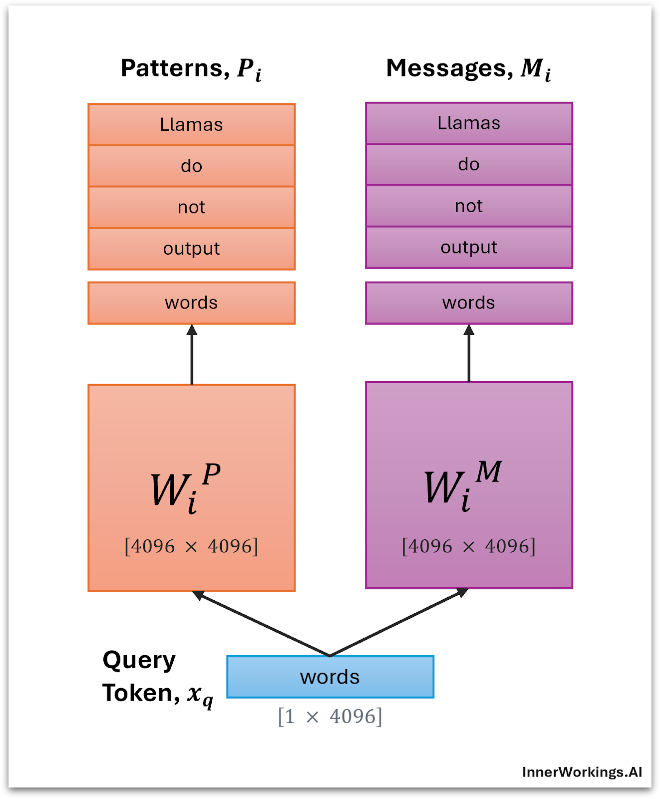
To add further clarity to the illustrations, I’ve included example matrix dimensions based on Llama 3 8B, which has an embedding size of 4,096.

The example text sequence is an important clarification about Llamas: “Llamas do not output words”.

In a given layer, Decoder Attention consists of two steps.

Step 1: Cache a Message

First, we project the input token to produce its pattern and message vectors, and add these to the cache.

Step 2: Attention Scoring

Next, multiply the input vector $x_q$ with all of the patterns in $P_i$ to see which patterns the input token is most similar to.

We apply the SoftMax function to normalize these values:

$\alpha_i = \mathrm{softmax}!\left(\frac{P^i {x_q}^{‘}}{\sqrt{d_k}}\right)$

This overall step is captured in the lefthand side of the below illustration:

Pattern Matching

The dot product can be thought of as a measure of similarity between the input and the patterns, as long as we recognize that the magnitude of the pattern vectors also influences the “matching”. Inspecting the magnitude of pattern vectors could be interesting!

Aside: What does the SoftMax do?

1. “Scales” the head output to ensure it always has the same magnitude, regardless of the current number of tokens.

2. Turns the matching into a competition between tokens–the similarity with a pattern is only significant in terms of how weak or strong it is in comparison to the other patterns.

Step 3: Aggregate Messages

For a given input vector, the output of attention head $i$ can now be elegantly viewed as the sum of the token messages, weighted by the attention scores.

$o_i = \alpha_i \,M_i $

where

• $\alpha_i \in \mathbb{R}^{1\times T}$ contains the attention scores for each token, and
• $M_i \in \mathbb{R}^{T\times d_{\text{model}}}$ are the tokens’ messsages.

This is shown in the righthand side of the earlier illustration:

The final output of the Attention block (including the residual connection) is the sum over the heads:

$x^\prime = x + \sum_i{\alpha_i M_i}$

Aside: The term “Aggregate” is also from Graph Neural Networks. It’s the step where a graph node sums up the weighted messages of its neighbors.

Decomposing

Here are the three formulations of a single Attention head in the style of the original Transformer paper.

We are applying attention to a single input (query) vector $x_q$, attending to a sequence of tokens in $X$, and this results in $o_i$, the re-projected (model space) output of $head_i$.

The first is the standard form, except that we’ve separated out the per-head output matrix, $W^O_i$

The second shows the terms re-arranged, but still decomposed.

Finally, the third shows the merged “patterns and messages” form.

Both the “refactored” and “merged” forms result in the creation of the pattern vectors $P_i$ and messages $M_i$, and I’ve indicated where these exist.

Compute Requirements

The purpose of the reformulations is just conceptual clarity, but it’s still worth noting the differences in compute involved.

The “refactored” form requires more compute than the “standard” form because the pattern matching and message scoring are done in model space.

The “merged” version requires even more compute because the word vectors are projected using full-size matrices.

Low Rank Matrices

The merged form can be easier to grasp and provides valuable insights into Attention; however, a downside is that it can obscure the crucial detail that these $W^P_i$ and $W^M_i$ matrices are very low rank.

In the same way that LoRA limits the impact that fine-tuning can have on the weight matrices, the low rank QK and VO decompositions imply that each head has a limited impact on the word vector.

Sub-spaces

The Transformer Circuits paper explains the significance of this in a more insightful way (if you can wrap your head around it!). Let’s use Llama 3 8B again, with its 4k embedding and head size of 128.

Each attention head “reads and writes to a 128-dimensional sub-space” of the word vector.

What’s a subspace? Here’s how I’m understanding it.

Picture a 3D point cloud of words, where you notice that there seems to be a particular direction in the cloud that correlates with how positive or negative the sentiment of the words are. You can highlight this by piercing the cloud with a line at the right location and angle.

You’ve found a subspace within your 3 dimensional embedding space! You can project words onto the line you found so that you have a feature capturing their sentiment.

If you project down to this sub-space, modify the sentiment value, and then project back up, the word will have moved up or down in the direction of that “sentiment” line.

You could find another line, and together they form a 2D subspace.

In Llama 3 8B, a head projects onto 128 “hyperlines” within the 4,096 dimensional embedding space.

Conclusion

Reformulating the Attention mechanism around patterns and messages isn’t meant to replace the standard approach–it’s intended to offer additional clarity for teaching, inspecting, and reasoning about our Transformer architectures.

I’m hoping this fresh perspective may inspire some new ideas (it certainly got my wheels turning!), and in Part 3 I’ll share how this formulation can be helpful in brainstorming alternative decompositions to improve efficiency–or at least help us better understand the ones we already use.