Patterns and Messages - Part 4 - Attention as a Dynamic Neural Network
When you reduce Attention down to two matrices instead of four, the pattern and message vectors represent a more familiar architecture–they form a neural network, whose neurons are created dynamically at inference time from the tokens.
This draws a nice parallel between the Feed Forward Neural Network and this “Attention Head Neural Network”.
The FFN is a large “static” neural network whose input and output weights are learned during training and then fixed. It uses the SwiGLU activation function.
The AHN is a dynamically built neural network whose input and output weights are created during inference by projecting the tokens. It uses the SoftMax activation function.
For a given head, the cached key vectors are the input neurons, and the cached value vectors are the output neurons.
It’s a little cleaner, though, when you use the pattern and message vectors, as I’ll show here.
by Chris McCormick
Contents
- Contents
- Feed Forward Neural Network
- Attention Head Neural Network
- Network Sizes
- Routing and Filtering
- Remember Low Rank
- Conclusion
- Appendix - Notation
Feed Forward Neural Network
First, just to highlight the similarity, here is how I might illustrate the FFN in Llama 3 8B, which has an embedding size of 4,096 and an FFN size (inner dimension) of 14,336.
I’ve included the dimensions because I find them helpful for understanding “what I’m looking at” in an illustration. Also, note that I’ve chosen to orient the “matrices” based on what’s convenient for the illustration rather than what’s required for correct matrix multiplication.
To evaluate the FFN:
The current input token is multiplied by the input neurons and their gates, resulting in an activation value for each neuron.
These activations are multiplied against their respective output neurons, which are summed to produce the output.

In the Attention network, the input weights are the pattern vectors and the output weights are the messages. I’ll go into more detail in the next section, but wanted to include this here for easy comparison.

I drew a box around the activations here to highlight that, unlike the FFN, they are normalized.
The attention neural network starts out small, but steadily grows in size as we process the sequence.
Also note that there are multiple of these per layer, corresponding to the number of heads, but only one FFN per layer.
Attention Head Neural Network
Within an attention head, when processing an input token, attention can be thought of in terms of two steps:
- Append a new input and output neuron to the network by projecting the input vector onto the Pattern and Messages spaces, respectively.
- Evaluate the network on the input vector.
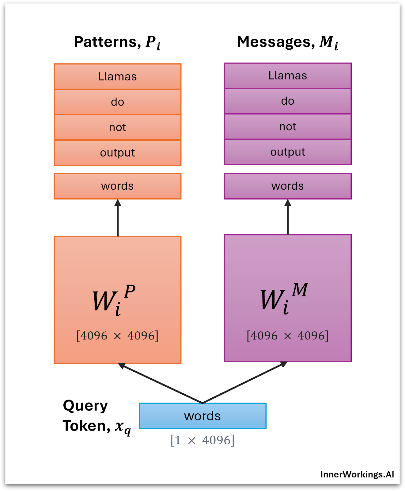
I’ve illustrated these two steps below. The text sequence is “Llamas do not output words” (unless they have version numbers! 😉), and the current input token is “words”.
The subscript $i$ refers to the head number, and I include it everywhere to reinforce that we are looking at a single head.
Step 1: Grow the Network
First, grow the network by projecting the input token to get its pattern vector and message vector, and append these to their respective matrices.
Step 2: Evaluate
Second, evaluate the updated network on that same input vector.
The output vector for this head and the others are all added to the current “residual stream”. The residual stream is simply the input embedding with all of the head outputs and FFN outputs added on top. I’ll explore this more in the next post.
Network Sizes
Which is bigger in the Transformer–the FFNs or the Attention blocks?
Let’s borrow the dimensions from Llama 3 8B again:
| Attribute | Size |
|---|---|
| Layers | 32 |
| Embedding | 4096 (4k) |
| Heads | 32 |
| Head Size | 128 |
| FFN Size | 14,336 (14k) |
(For simplicity, let’s ignore GQA and assume it’s vanilla attention)
Number of Learned Parameters
The FFNs have 3 matrices–input, output, and gate, with $56M$ parameters each, so $168M$ total per layer.
The Attention blocks have 4 square projection matrices, $16M$ parameters each, so $64M$ parameters total per layer.
Compared to the Attention Projection matrices, the FFN has almost 3x as many parameters!
But what about this “Attention Head Network” that we’ve defined?
AHN vs. FFN Size
Comparing the number of parameters and compute cost of the AHNs versus the FFNs is tricky, because we employ tricks like matrix decomposition and GQA to cut down the cost of Attention.
I think it’s interesting, though, to compare the two in terms of number of neurons, or output neurons to be specific.
Attention Head Networks:
Each token produces a message for each head–these are the output neurons of the AHN.
With 32 layers and 32 heads, there are 1,024 heads total, which means there 1,024 messages per token.
Feed Forward Networks:
The number of FFN outputs is fixed at 32 layers x $14k$ = 494k output neurons.
Comparison:
The massive pre-trained weights of the FFNs dominate the model initially, but each new token adds another 1,024 neurons to our dynamically built Attention Head Networks.
The AHNs surpass the FFNs in size once the sequence length grows past 494 tokens!
At the maximum sequence of 8,192 tokens, there are 8M messages vs. 494K output neurons.
Efficiency Insights
This alternate framing provides another way of looking at a problem we’re already very aware of–that attention gets increasingly expensive as we add tokens.
Perhaps it’s a fresh perspective that can inspire creativity–what ideas could we borrow from FFNs to try applying to these AHNs?
For example, another way to frame Group Query Attention is as a form of “weight tying”–groups of four AHNs share output weights.
With FFNs we have an understanding and techniques around there being ‘unneccessary neurons’. I haven’t explored the research in this area yet, but here are some thoughts I had around applying those insights to AHNs.
Routing and Filtering
Token Filtering
These AHNs are clearly flexibile–they manage to function whether they contain just 5 neurons, or 5,000.
As we build each of them–does every token really need to be added to every head?
I’m curious whether the message projections, $W^M_i$, have learned to recognize when a token isn’t relevant, and so they record a message $m_i$ that is just “harmless noise”.
If so, could we detect this condition instead, and refrain from adding the token to that AHN?
Routing
Seeing the heads as neural networks draws the comparison to Mixture of Experts. MoE works by clustering related neurons (based on their input neurons) so that we can route inputs to only, e.g., 8 clusters by comparing them to the cluster centroids.
The corollary here is the pattern vectors / key vectors, which serve as the input neurons.
Could we partition the KV cache to store the keys in clusters, and use their centroids to route query vectors to only the top matching groups of keys?
Gating
We’re dynamically creating input and output neurons; should we be dynamically creating gates for them as well?
Gates feel highly intuitive to me. They seem to separate out the task of “is this input neuron relevant?” so that the neuron can focus on “how much of my output should be added or subtracted from the result?”.
I think we use SoftMax instead partly because it handles a key problem–we don’t want the magnitude of the output to keep growing as we add more neurons to the AHNs. The SoftMax normalizes the scores to mitigate this.
Instead of normalizing–in the same way that LoRA divides the outputs by the square root of the rank, could we divide the head outputs by the square root of the number of neurons?
Inspiration
That’s all just speculation, and may have already been explored, but I like how this perspective “got my wheels turning”!
Remember Low Rank
If there’s a drawback to this perspective (and to patterns and messages in general), it’s that it hides the fact that the neurons are low rank, compared to the FFNs.
It’s important to remember that these Attention Head Networks have been “bottlenecked” through low rank decomposition so that they only modify a particular “subpace” of the token vector.
In the same way that LoRA limits how much impact the fine-tuning process has on the model weights, each AHN has a far lower impact on the word vector compared to the FFN.
Conclusion
Collapsing down from “QKVO” to “PM” helps us see attention from a new angle, as dynamically building a neural network from each new token.
This framing encourages us to ask questions like:
- Does every context token need to add a message to every head?
- Does every input token need to be compared to every context token?
- Should we gate the scores instead of normalizing them?
In the next post, we’ll look at another concept from Mechanistic Interpretability called “The Residual Stream”, which pulls the concepts in this post together to describe the behavior of a layer and the Transformer overall.
Appendix - Notation
For those who’d prefer a mathematical definition…
In a Decoder text generation model, the current input vector is used in all three roles, $x_q = x_k = x_v $, but I’ll keep them separate just to help us map things back to what we’re used to.
Step 1: Grow the Network
The pattern vector $p_i$ is produced by projecting the key token onto the Pattern space:
$p_i = x_kW^P_i$
The message vector $m_i$ is produced by projecting the value token onto the Message space:
$m_i = x_vW^M_i$
These get appended to the vectors in the cache (the left arrow refers to “updating” / replacing the matrix):
$P_i \gets \text{Concat}(P_i, \; p_i)$
$M_i \gets \text{Concat}(M_i, \; m_i)$
Step 2: Evaluate the Network
Calculate the activations by multiplying the query token against all of the pattern vectors, and then normalizing those activations with the SoftMax.
$\alpha_i = \text{SoftMax} \left(\frac{x_q P_i^{‘}}{\sqrt{d^{h}}} \right)$
And then the output of the network (i.e., the output of the Attention head) is:
$o_i = \alpha_iM_i$