Reading and Writing with Projections

Transformers store, retrieve, and modify data along different feature directions in their model space, via projections.

I’m finding that building some better intuition around what this actually means can be a powerful tool for reasoning about LLM architecture.

Probably the most intriguing quality of ‘feature directions’ is that a model with an embedding size of 4,096 is able to stuff more than 4K features into that space.

To explore this notion, let’s see if we can use this same Transformer math to store three settings from your speakers–bass, volume, and treble–into 2 dimensions.

There are some surprising quirks to how a model stores even just 2 values in 2 dimensions, though, so let’s cover that simpler case first.

by Chris McCormick

Contents

• Contents
• Encoding & Decoding
• Model Directions
• Modifying Values
• More Features than Dimensions
  • The Blessing of Dimensionality
• Features in Transformers
• Conclusion

Encoding & Decoding

Say you’ve got your base at 8 (unce, unce, unce…) and volume at 5.

(For the math, let’s call this 0.8 and 0.5).

To store these in a two dimensional vector, the sensible choice is to put them in a vector that just looks like an array: $x = [0.8, 0.5]$.

But we need to start thinking differently, in terms of data being stored in feature directions.

When we write $x = [0.8, 0.5]$, we’re actually storing those values along two particular feature directions: bass is in the direction of the vector $v_1 = [0, 1]$ and volume in the direction of $v_2 = [1, 0]$

To facilitate reading and writing, we combine $v_1$ and $v_2$ as column vectors in a projection matrix, $W$.

To encode our data, we calculate $x^v = W x^T$:

Then, to decode and recover $x$, we calculate $x^vW$:

Here’s a plot of our chosen feature directions, the encoded data point, and how it projects onto each of the directions:

Input Settings:
   [0.8 0.5]

Feature Directions:
  bass  : [1. 0.]
  volume: [0. 1.]

Encoded settings:
   [0.8 0.5]

Decoded settings:
   [0.8 0.5]

Clearly this is rather pointless so far (other than to give you a small math headache). Our feature directions are aligned with axes and there’s no difference in the encoded and decoded versions.

Things change, though, once we dive into the world of neural networks.

Model Directions

Here’s the first insight we need to establish–our models generally don’t have any reason to pick those nice, axis-aligned directions.

Any two arbitrary directions will do, the only “requirement” is that they be perpendicular (“orthogonal”).

Orthogonal Directions

The reason you want them orthogonal is that it means you can store / modify them without interfering with each other. We can change the volume and the bass won’t be affected.

The model has to learn these directions, though, so:

1. They probably won’t align with axes, and
2. They probably won’t be perfectly orthogonal.

As an example, let’s say the model ends up storing bass along the direction $[0.94, 0.34]$ and volume along $[-0.36, 0.93]$–two directions that are very close to, but not perfectly, orthogonal.

We can repeat our earlier plot with these new directions. The fact that they’re not perfectly orthogonal results in a tiny bit of intereference, causing some slight recovery error.

Input Settings:
   [0.8 0.5]

Feature Directions:
  bass  : [0.94 0.34]
  volume: [-0.36  0.93]

Encoded settings:
   [0.57 0.74]

Decoded settings:
   [0.79 0.49]

Consequences

So the math all works exactly as it did in the axis-aligned case, except now:

1. Our encoded vector is incomprehensible (see below), and
2. Imperfect directions leads to some interference and error in the values.

Modifying Values

Let’s cover one more Transformer-related detail before we try packing in that third speaker setting.

We’ve seen how to read (decode) values, and how to store (encode) them. However, Transformers don’t encode values–they update them.

Transformer blocks output an amount to adjust the input by. For example, the FFN calculates:

$x = x + \text{FFN}(x)$

(i.e., the FFN calculates a “residual” vector)

Encoding an Adjustment

Let’s say the neighbors are complaining, so we relent and turn the bass down to 6.

Rather than encode the new values [0.6, 0.5], we’ll encode an adjustment to make.

Our original values were [0.8, 0.5] and we want to make the adjustment [-0.2, 0]. so we encode that as:

adjustment   = np.array([-0.2, 0.0])       # Turn the bass down by 2.

adjustment_enc = proj @ adjustment.T

print("Adj. to make:", adjustment)
print("Encoded adj.:", adjustment_enc)

Adj. to make: [-0.2  0. ]
Encoded adj.: [-0.19 -0.07]

Add it to our encoded vector:

enc_settings = settings_enc + adjustment_enc

print("Updated encoding:", enc_settings)

Updated encoding: [0.38 0.67]

And then we can recover (with slight error) the updated settings by decoding:

dec_settings = enc_settings @ proj

print("Recovered settings:", dec_settings)

Recovered settings: [0.59 0.49]

Now we have the fundamental tools for working with feature directions, and we’re ready to move on to the original challenge.

More Features than Dimensions

Again–all of this encoding and decoding is pretty obnoxious when you could just store those two features along the directions [1, 0] and [0, 1].

But we’ve unlocked something really cool. We now have a way to take our settings / data values / features and store them in a vector just by choosing directions to encode them along–and the math allows you to choose as many directions as you want! You’re not limited to just 2.

That’s exactly what our models do–a transformer with an embedding size of 4,096 is packing far more data values in the token vector than just 4K.

So let’s try this out ourselves!

Bass, Volume, and Treble

We established that we can choose any arbitrary directions to store data along, we just want them to be as orthogonal as possible so that they don’t interfere with each other.

That means we want to spread the three feature directions out as much as possible. In 2 dimensions, the best we can do is to make them each 120 degrees apart.

Let’s see what happens when we encode our speaker settings now–bass at 8 (to hell with the neighbors), volume at 5, treble at 4:

Input Settings:
   [0.8 0.5 0.4]

Feature Directions:
  bass  : [0.98 0.17]
  volume: [-0.64  0.77]
  treble: [-0.34 -0.94]

Encoded settings:
   [0.33 0.15]

Decoded settings:
   [ 0.35 -0.1  -0.25]

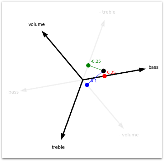
Ok… So that didn’t go very well. The recovery is so bad that some of the settings ended up negative (we broke the knobs on our stereo! 😭).

If adding just one extra feature broke everything, how do Transformers get away with adding thousands?

The Blessing of Dimensionality

Our giant models benefit from “the blessing of dimensionality”. It turns out that the more dimensions you have to work with, the more you can overload them without terrible interference.

A length 4,096 embedding is so high dimensional that you can pick any 2 random directions, and they’ll likely be pretty close to orthogonal.

import numpy as np

# Create two randomly initialized vectors with length 4,096
vec1 = np.random.randn(4096)
vec2 = np.random.randn(4096)

# Set numpy print precision to 2 decimal points
np.set_printoptions(precision=2)

# Normalize the vectors
vec1 = vec1 / np.linalg.norm(vec1)
vec2 = vec2 / np.linalg.norm(vec2)

# Calculate the dot product of the two vectors
dot_product = np.dot(vec1, vec2)

print(f"Dot product between two random 4K vectors (a value of 0.0 is orthogonal):")
print(f"  {dot_product:.4}", )

Dot product between two random 4K vectors (a value of 0.0 is orthogonal):
  -0.01718

Transformers / Deep Neural Networks have the further advantage of being pretty noise tolerant, and they can survive with more interference than we might allow in other applications.

Let’s see if we can leverage this “blessing” ourselves by adding more dimensions.

To stick with our speaker system example, let’s try encoding the settings of a large equalizer that has 30 sliders.

We’ll pick 30 feature directions, but pack them into 29 dimensions to see how bad the interference is.

(Note: Finding these orthogonal-as-possible directions is non-trivial–the code below is going to learn some for us!)

# Repulsion-based cosine similarity minimization using NumPy
np.random.seed(42)

# Parameters
n_features = 30
dim = 29
num_iters = 5000
lr = 0.05

# Start with random unit vectors (columns shape [dim, n_features])
vecs = np.random.randn(dim, n_features)
vecs /= np.linalg.norm(vecs, axis=0, keepdims=True)

# Optimization loop
for _ in range(num_iters):
    # Cosine similarities
    dot = vecs.T @ vecs
    np.fill_diagonal(dot, 0)

    # Compute repulsion gradients
    grad = vecs @ dot

    # Gradient descent step
    vecs -= lr * grad

    # Re-normalize to unit vectors
    vecs /= np.linalg.norm(vecs, axis=0, keepdims=True)

# Compute final cosine similarity stats
cos_sim_final = vecs.T @ vecs
np.fill_diagonal(cos_sim_final, 0)
max_sim_final = np.max(np.abs(cos_sim_final))
mean_sim_final = np.mean(np.abs(cos_sim_final))

print("Similarity between any two vectors (ideal is 0.0):")
print(f"  Average: {mean_sim_final:.3}")
print(f"    Worst: {max_sim_final:.3}")

Similarity between any two vectors (ideal is 0.0):
  Average: 0.0333
    Worst: 0.0345

GPT helped me build a cute visualization for this below.

The grey knobs show the original settings, and the green knobs are the recovered settings after encoding and decoding, to illustrate the interference.

There’s still a fair amount of interference, but the results are certainly much more sensible than our 3-into-2 example.

Let’s take it further.

Even More Dimensions

What if we have 512 dimensions to work with, and pack in 513 features?

To illustrate this, I found 513 directions to use, and then made sure to store data along all of them so that there’s still interference, but we’ll just show 30.

Much better!

Side Note:

I will say–I expected the interference to be lower given that we only added a single feature to the vector.

I did use uniformly random values for the settings, whereas the values in our models tend to be normally distributed (and maybe normalized as well?)–perhaps that is important?

Also, I did store values along every single direction–perhaps a critical piece is that a given vector rarely carries around that many feature values all at once?

Features in Transformers

I think it’s fair to say that a given Transformer model has learned a large underlying feature-direction matrix, with more columns than rows (i.e., more directions than the length of the token embedding).

But do the various weights and activations we see in the model correspond to those features?

Unfortunately, no. Because these operations are linear, they can be combined!

Instead of writing to one of these “true” feature directions directly, the model composites them by combining other vectors.

The model can read the value stored along $v$ by executing $xv$, but it can also read it by calculating $x(a + b + c)$ if those three vectors sum up to $v$.

Similarly, the model could be adjusting $v_1$ by 0.2 and $v_2$ by -0.1, but all we get to see is the combination of multiple such updates, making them hard to tease apart.

And, as we can see clearly in simpler machine learning models, additional meaningful features can exist as linear or non-linear combinations of these ~orthogonal directions.

Quite a lot to untangle when doing interpretability research!

Conclusion

Thinking through all of this has definitely given me some stronger intuition about projections beyond just “dimensionality reduction” and “feature extraction”.

It also leads in to many other interesting topics, like what “low-rank” really means and why it matters, and going deeper into the complex terminology and insights of interpretability (like “superposition”!).

Hopefully more on those soon!