The Gaussian Kernel
Each RBF neuron computes a measure of the similarity between the input and its prototype vector (taken from the training set). Input vectors which are more similar to the prototype return a result closer to 1. There are different possible choices of similarity functions, but the most popular is based on the Gaussian. Below is the equation for a Gaussian with a one-dimensional input.

Where x is the input, mu is the mean, and sigma is the standard deviation. This produces the familiar bell curve shown below, which is centered at the mean, mu (in the below plot the mean is 5 and sigma is 1).

The Gaussian function is complicated and includes many terms; we’ll dig into each of them in the following sections. But first, there are some important observations we can make just from the shape of the function.
Note that each RBF neuron will produce its largest response when the input is equal to the prototype vector. This allows to take it as a measure of similarity, and sum the results from all of the RBF neurons.
As we move out from the prototype vector, the response falls off exponentially. Recall from the RBFN architecture illustration that the output node for each category takes the weighted sum of every RBF neuron in the network–in other words, every neuron in the network will have some influence over the classification decision. The exponential fall off of this Gaussian function, however, means that the neurons whose prototypes are far from the input vector will actually contribute very little to the result.
Euclidean Distance
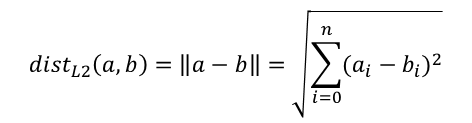
The Gaussian function is based, first of all, on the Euclidean distance between the input vector and the prototype. You probably remember the Euclidean distance from geometry.
In higher dimensions, this is generalized to:
It’s useful to plot this function to see its shape. For a one-dimensional input, the Euclidean distance has a ‘V’ shape. Below is the plot of the Euclidean distance between x and 0.
 In Google, type “plot y = sqrt(x^2)” to produce this plot
For a two-dimensional input, it becomes a cone. The below plot shows the Euclidean distance between (x, y) and (0, 0).
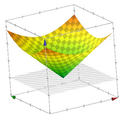 In Google, type “plot z = sqrt(x^2 + y^2)” to produce this plot
The first thing you’ll notice about the Euclidean distance is that it produces the inverse of the response we want–we want the neuron to produce it’s largest response when the input is equal to the prototype. We’ll deal with that in the next section.
The Gaussian function is based on the squared Euclidean distance. Note that squaring the Euclidean distance is the same as just removing the square root term. This leads to the (x - mu)^2 term in the equation for the one dimensional Gaussian. For a one-dimensional input, the squared Euclidean distance is just the parabola y = x^2

For two-dimensions: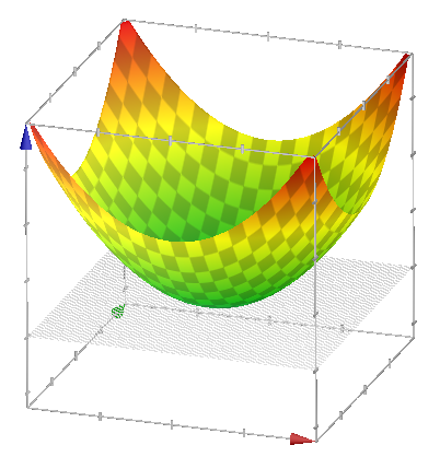 In Google, type “plot z = x^2 + y^2” to produce this plot
The Exponential
The next part of the equation we’ll look at is the negative exponent. Adding in the negative exponent gives us the following equation, plotted below as the blue line. I’ve used the double bar notation here for expressing the Euclidean distance between x and mu. For comparison, the red line is given by
 In Google, type “plot y = exp(-(x^2)) and y = -x^2 + 1” to produce this plot
The negative exponent falls off more gradually and also never reaches 0. This is desirable, since we don’t want the neuron to produce a negative response just because it is too far from an input of the same category.
The Variance
The Gaussian equation also contains two coefficients which are based on the parameter sigma.
The inner coefficient controls the width of the bell curve. The sigma squared term is known as the “variance” of the distribution, since it dictates how much the distribution varies from the mean. For the RBFN, we will encapsulte the entire 1 / (2 * sigma^2) term into a single coefficient value; we’ll use the Greek letter beta to represent this coefficient.

The below plot shows the effect of different values of beta on the curve.

The beta coefficient is important for controlling the influence of the RBF neuron. Each RBF neuron provides most of its response in a circular region around its center. The size of this circle is controlled by beta.
The Gaussian equation contains one final coefficient, 1 / (sigma * sqrt(2 * pi)). This outer coefficient just controls the height of the distribution. Recall from the RBF network architecture that we will apply a weight to the output of every RBF neuron. This weight is redundant with the outer coefficient of the Gaussian equation, so the coefficient is omitted from the equation for the RBF neuron’s activation function.