Radial Basis Function Network (RBFN) Tutorial

A Radial Basis Function Network (RBFN) is a particular type of neural network. In this article, I’ll be describing it’s use as a non-linear classifier.

Generally, when people talk about neural networks or “Artificial Neural Networks” they are referring to the Multilayer Perceptron (MLP). Each neuron in an MLP takes the weighted sum of its input values. That is, each input value is multiplied by a coefficient, and the results are all summed together. A single MLP neuron is a simple linear classifier, but complex non-linear classifiers can be built by combining these neurons into a network.

To me, the RBFN approach is more intuitive than the MLP. An RBFN performs classification by measuring the input’s similarity to examples from the training set. Each RBFN neuron stores a “prototype”, which is just one of the examples from the training set. When we want to classify a new input, each neuron computes the Euclidean distance between the input and its prototype. Roughly speaking, if the input more closely resembles the class A prototypes than the class B prototypes, it is classified as class A.

RBF Network Architecture

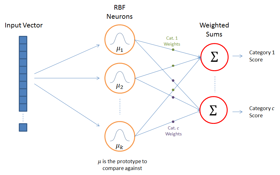
The above illustration shows the typical architecture of an RBF Network. It consists of an input vector, a layer of RBF neurons, and an output layer with one node per category or class of data.

The Input Vector

The input vector is the n-dimensional vector that you are trying to classify. The entire input vector is shown to each of the RBF neurons.

The RBF Neurons

Each RBF neuron stores a “prototype” vector which is just one of the vectors from the training set. Each RBF neuron compares the input vector to its prototype, and outputs a value between 0 and 1 which is a measure of similarity. If the input is equal to the prototype, then the output of that RBF neuron will be 1. As the distance between the input and prototype grows, the response falls off exponentially towards 0.  The shape of the RBF neuron’s response is a bell curve, as illustrated in the network architecture diagram.

The neuron’s response value is also called its “activation” value.

The prototype vector is also often called the neuron’s “center”, since it’s the value at the center of the bell curve.

The Output Nodes

The output of the network consists of a set of nodes, one per category that we are trying to classify. Each output node computes a sort of score for the associated category. Typically, a classification decision is made by assigning the input to the category with the highest score.

The score is computed by taking a weighted sum of the activation values from every RBF neuron. By weighted sum we mean that an output node associates a weight value with each of the RBF neurons, and multiplies the neuron’s activation by this weight before adding it to the total response.

Because each output node is computing the score for a different category, every output node has its own set of weights. The output node will typically give a positive weight to the RBF neurons that belong to its category, and a negative weight to the others.

RBF Neuron Activation Function

Each RBF neuron computes a measure of the similarity between the input and its prototype vector (taken from the training set). Input vectors which are more similar to the prototype return a result closer to 1. There are different possible choices of similarity functions, but the most popular is based on the Gaussian. Below is the equation for a Gaussian with a one-dimensional input.

Where x is the input, mu is the mean, and sigma is the standard deviation. This produces the familiar bell curve shown below, which is centered at the mean, mu (in the below plot the mean is 5 and sigma is 1).

The RBF neuron activation function is slightly different, and is typically written as:

In the Gaussian distribution, mu refers to the mean of the distribution. Here, it is the prototype vector which is at the center of the bell curve.

For the activation function, phi, we aren’t directly interested in the value of the standard deviation, sigma, so we make a couple simplifying modifications.

The first change is that we’ve removed the outer coefficient, 1 / (sigma * sqrt(2 * pi)). This term normally controls the height of the Gaussian. Here, though, it is redundant with the weights applied by the output nodes. During training, the output nodes will learn the correct coefficient or “weight” to apply to the neuron’s response.

The second change is that we’ve replaced the inner coefficient, 1 / (2 * sigma^2), with a single parameter ‘beta’. This beta coefficient controls the width of the bell curve. Again, in this context, we don’t care about the value of sigma, we just care that there’s some coefficient which is controlling the width of the bell curve. So we simplify the equation by replacing the term with a single variable.

RBF Neuron activation for different values of beta

There is also a slight change in notation here when we apply the equation to n-dimensional vectors. The double bar notation in the activation equation indicates that we are taking the Euclidean distance between x and mu, and squaring the result. For the 1-dimensional Gaussian, this simplifies to just (x - mu)^2.

It’s important to note that the underlying metric here for evaluating the similarity between an input vector and a prototype is the Euclidean distance between the two vectors.

Also, each RBF neuron will produce its largest response when the input is equal to the prototype vector. This allows to take it as a measure of similarity, and sum the results from all of the RBF neurons.

As we move out from the prototype vector, the response falls off exponentially. Recall from the RBFN architecture illustration that the output node for each category takes the weighted sum of every RBF neuron in the network–in other words, every neuron in the network will have some influence over the classification decision. The exponential fall off of the activation function, however, means that the neurons whose prototypes are far from the input vector will actually contribute very little to the result.

If you are interested in gaining a deeper understanding of how the Gaussian equation produces this bell curve shape, check out my post on the Gaussian Kernel.

Example Dataset

Before going into the details on training an RBFN, let’s look at a fully trained example.

In the below dataset, we have two dimensional data points which belong to one of two classes, indicated by the blue x’s and red circles. I’ve trained an RBF Network with 20 RBF neurons on this data set. The prototypes selected are marked by black asterisks.

We can also visualize the category 1 (red circle) score over the input space. We could do this with a 3D mesh, or a contour plot like the one below. The contour plot is like a topographical map.

The areas where the category 1 score is highest are colored dark red, and the areas where the score is lowest are dark blue. The values range from -0.2 to 1.38.

I’ve included the positions of the prototypes again as black asterisks. You can see how the hills in the output values are centered around these prototypes.

It’s also interesting to look at the weights used by output nodes to remove some of the mystery.

For the category 1 output node, all of the weights for the category 2 RBF neurons are negative:

-0.79934
-1.26054
-0.68206
-0.68042
-0.65370
-0.63270
-0.65949
-0.83266
-0.82232
-0.64140

And all of the weights for category 1 RBF neurons are positive:

0.78968
0.64239
0.61945
0.44939
0.83147
0.61682
0.49100
0.57227
0.68786
0.84207

Finally, we can plot an approximation of the decision boundary (the line where the category 1 and category 2 scores are equal).

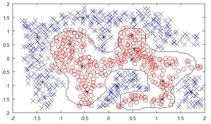
To plot the decision boundary, I’ve computed the scores over a finite grid. As a result, the decision boundary is jagged. I believe the true decision boundary would be smoother.

Training The RBFN

The training process for an RBFN consists of selecting three sets of parameters: the prototypes (mu) and beta coefficient for each of the RBF neurons, and the matrix of output weights between the RBF neurons and the output nodes.

There are many possible approaches to selecting the prototypes and their variances. The following paper provides an overview of common approaches to training RBFNs. I read through it to familiarize myself with some of the details of RBF training, and chose specific approaches from it that made the most sense to me.

Selecting the Prototypes

It seems like there’s pretty much no “wrong” way to select the prototypes for the RBF neurons. In fact, two possible approaches are to create an RBF neuron for every training example, or to just randomly select k prototypes from the training data. The reason the requirements are so loose is that, given enough RBF neurons, an RBFN can define any arbitrarily complex decision boundary. In other words, you can always improve its accuracy by using more RBF neurons.

What it really comes down to is a question of efficiency–more RBF neurons means more compute time, so it’s ideal if we can achieve good accuracy using as few RBF neurons as possible.

One of the approaches for making an intelligent selection of prototypes is to perform k-Means clustering on your training set and to use the cluster centers as the prototypes. I won’t describe k-Means clustering in detail here, but it’s a fairly straight forward algorithm that you can find good tutorials for.

When applying k-means, we first want to separate the training examples by category–we don’t want the clusters to include data points from multiple classes.

Here again is the example data set with the selected prototypes. I ran k-means clustering with a k of 10 twice, once for the first class, and again for the second class, giving me a total of 20 clusters. Again, the cluster centers are marked with a black asterisk ‘*’.

I’ve been claiming that the prototypes are just examples from the training set–here you can see that’s not technically true. The cluster centers are computed as the average of all of the points in the cluster.

How many clusters to pick per class has to be determined “heuristically”. Higher values of k mean more prototypes, which enables a more complex decision boundary but also means more computations to evaluate the network.

Selecting Beta Values

If you use k-means clustering to select your prototypes, then one simple method for specifying the beta coefficients is to set sigma equal to the average distance between all points in the cluster and the cluster center.

Here, mu is the cluster centroid, m is the number of training samples belonging to this cluster, and x_i is the ith training sample in the cluster.

Once we have the sigma value for the cluster, we compute beta as:

Output Weights

The final set of parameters to train are the output weights. These can be trained using gradient descent (also known as least mean squares).

First, for every data point in your training set, compute the activation values of the RBF neurons. These activation values become the training inputs to gradient descent.

The linear equation needs a bias term, so we always add a fixed value of ‘1’ to the beginning of the vector of activation values.

Gradient descent must be run separately for each output node (that is, for each class in your data set).

For the output labels, use the value ‘1’ for samples that belong to the same category as the output node, and ‘0’ for all other samples. For example, if our data set has three classes, and we’re learning the weights for output node 3, then all category 3 examples should be labeled as ‘1’ and all category 1 and 2 examples should be labeled as 0.

RBFN as a Neural Network

So far, I’ve avoided using some of the typical neural network nomenclature to describe RBFNs. Since most papers do use neural network terminology when talking about RBFNs, I thought I’d provide some explanation on that here. Below is another version of the RBFN architecture diagram.

Here the RBFN is viewed as a “3-layer network” where the input vector is the first layer, the second “hidden” layer is the RBF neurons, and the third layer is the output layer containing linear combination neurons.

One bit of terminology that really had me confused for a while is that the prototype vectors used by the RBFN neurons are sometimes referred to as the “input weights”. I generally think of weights as being coefficients, meaning that the weights will be multiplied against an input value. Here, though, we’re computing the distance between the input vector and the “input weights” (the prototype vector).

Example MATLAB Code

I’ve packaged up the example dataset in this post and my MATLAB code for training an RBFN and generating the above plots. You can find it here.