Kernel Regression

Having learned about the application of RBF Networks to classification tasks, I’ve also been digging in to the topics of regression and function approximation using RBFNs. I came across a very helpful blog post by Youngmok Yun on the topic of Gaussian Kernel Regression.

Gaussian Kernel Regression is a regression technique which interestingly does not require any iterative learning (such as gradient descent in linear regression).

I think of regression as simply fitting a line to a scatter plot. In Andrew Ng’s machine learning course on Coursera, he uses the example of predicting a home’s sale value based on its square footage.

Note that the data points don’t really lie on the line. Regression allows for the fact that there are other variables or noise in the data. For example, there are many other factors in the sale price of a home besides just the square footage.

Gaussian Kernel Regression is a technique for non-linear regression. I like the dataset Youngmok Yun used in his post, so I’m going to reuse it here.

The black line represents our original function given by the following equation:

 The blue points are taken from this function, but with random noise added to make it interesting. Using only the blue data points, Gaussian Kernel Regression arrives at the approximated function given by the red line. Pretty impressive!

Here’s another fun example in three dimensions. Below is a plot of what’s known as the “sombrero” function. The first plot shows the original sombrero function. In the second plot I’ve added random noise to the data points. The third plot shows the result of using Gaussian Kernel Regression to recover the original function.

Approximation With Weighted Averaging

Before we dive into the actual regression algorithm, let’s look at the approach from a high level.

Let’s say you have the following scatter plot, and you want to approximate the ‘y’ value at x = 60. We’ll call this our “query point”.

How would you go about it? One way would be to look at the data points near x = 60, say from x = 58 to x = 62, and average their ‘y’ values. Even better would be to somehow weight the values based on their distance from our query point, so that points closer to x = 60 got more weight than points farther away.

This is precisely what Gaussian Kernel Regression does–it takes a weighted average of the surrounding points.

Say we want to take the weighted average of three values: 3, 4, and 5.  To do this, we multiply each value by its weight (I’ve chosen some arbitrary weights: 0.2, 0.4, and 0.6), take the sum, then divide by the sum of the weights:

More generally, the weighted average is found as:

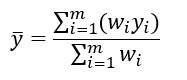
Where w__i is the weight to assign to value _y__i, and _m is number of values in the set.

Note that the weight values don’t have to add up to one. In fact, the magnitude of the values isn’t important, only the ratios.

Gaussian Kernel

To compute the weight values to use in our regression problem, we’re going to use the Gaussian function:

Where mu is the mean and sigma squared is the variance. The outer term of this function 1 / (sigma * sqrt(2 * pi))) will cancel out when we compute the weighted average, so we will omit it, leaving us with:

With sigma = 1 and mu = 0, this function has the following plot:

This function has exactly the behavior we want for computing our weight values if  we replace ‘mu’ with our query point. The function will produces its highest value when the distance between the data point and the query point is zero. For data points farther from the query, the weight value will fall off exponentially. When performing kernel regression, we will actually compute the weighted average over every training point; however, as you can see the from the plot of the Gaussian, only data points near the query are going to contribute significantly to the result.

To arrive at the final equation for Gaussian Kernel Regression, we’ll start with the equation for taking a weighted average:

And replace the weight values _w__i with our Gaussian “kernel function”:

This kernel function computes the weight to apply for data point x__i based on its distance from our query point _x*.

Substituting K for w, we have our final equation for approximating the output value y* at the query point x*:

To plot the approximated function, you would evaluate the above equation over a range of query points.

The above equation is the formula for what is more broadly known as Kernel Regression. We are simply applying Kernel Regression here using the Gaussian Kernel.

Gaussian Variance

An important parameter of Gaussian Kernel Regression is the variance, sigma^2. Informally, this parameter will control the smoothness of your approximated function. Smaller values of sigma will cause the function to overfit the data points, while larger values will cause it to underfit. The below plots show the result of using three different values of sigma: 0.5, 5, and 50.

Sigma controls the width of the Gaussian, so a larger value of sigma will incorporate farther away points into the averaging, resulting in a smoother result.

I haven’t read up on formal approaches for selecting the sigma value. However, a common technique for parameter selection in machine learning is to use an experimentation approach. First, create a hold-out validation set and select the parameter value which provides the best performance on the validation data. To measure the “performance” in this case, you might try the mean squared error between the validation outputs and the approximated outputs.

Relation To RBF Networks

It is interesting to note that Gaussian Kernel Regression is equivalent to creating an RBF Network with the following properties:

1. Every training example is stored as an RBF neuron center.

2. The beta coefficient (based on sigma) for every neuron is set to the same value.

3. There is one output node.

4. The output weight for each RBF neuron is equal to the output value of its data point.

5. The output of the RBFN must be normalized by dividing it by the sum of all of the RBF neuron activations.

You can read my post on RBF Networks for classification here.

Octave / Matlab Code

The following zip file contains two example scripts: ‘run2DExample.m’ and ‘run3DExample.m’ which run regression on the datasets in this post.

Example Code

The implementation of regression in run2DExample is easier to understand, but is limited to 2D datasets. In the 3D example (with the sombrero function) the implementation is generalized to work for inputs with any number of dimensions.

Again, thank you to Youngmok Yun; I started with his example code and am using his 2D dataset.

Additional References

• Kernel Regression is a form of Non-Parametric Regression.